Highlights

• Obesity rises from multiple causes and factors including lifestyle and transportation choices.
• Use of personal transport and a sedentary lifestyle are leading causes of the current obesity rates.
• The decision tree (DT) model accurately classifies and predicts obesity factors with 90.36% accuracy.
• Machine learning (ML) identifies key obesity factors, thus aiding public health awareness which helps to reduce obesity rates.

1. INTRODUCTION

Significant health risks result from the buildup of excess fat that leads to overweight and obesity. According to the criteria set by the World Health Organization (WHO), a body mass index (BMI) of over 25 is considered overweight and a BMI of over 30 is considered obese [1]. The global scope of this health issue was highlighted in 2017, when problems associated with being overweight or obese were blamed for almost 4 million deaths. The WHO reports concerning trends that show an increase in overweight and obesity rates, particularly among kids and teens, with percentages rising from 4% to 18% between the years 1975 and 2016 [1].

Pakistan, with the 9^th highest rate of obesity worldwide, has faced serious public health challenges in recent years. Numerous causes contribute to this concerning figure but the Pakistani population's choices for mobility garner particular attention [2]. The increasing use of cars and bicycles, even for short trips, has been identified as a significant factor in the nation's rising obesity rates. Short-distance walking has become less common as people choose to drive instead of walking, since it is more convenient. People have adopted gradually a more sedentary lifestyle as a result of this change in transportation preferences, ignoring the physical activity that comes with walking.

As a result, inadequate physical activity has emerged as a critical component in the country's obesity pandemic [2, 3]. The predominant mode of transportation in Pakistan is indicative of a reduction in the levels of physical activity. The trend toward using cars and bicycles to travel distances that people have historically traversed on foot is indicative of a larger shift in the society toward a more sedentary way of life. This change not only brings up pressing health issues but also emphasizes how crucial it is to look into the structural variables affecting travel decisions.

Literature shows that longer screen time contributes more to complex issues of obesity and also leads to a lack of physical exercise. The complex web of factors contributing to weight gain includes the correlation between excessive screen time and unhealthy eating patterns, such as eating more junk food, sugar-filled beverages, and unhealthy snacks, while consuming fewer fruits and vegetables [2]. This association is also influenced by targeted food advertising, careless snacking during screen time, and the potential masking of fullness signals.

An additional aspect of the problem is insufficient transportation infrastructure. Walking is not as preferred as motorized transportation, indicating a tendency in the society where convenience frequently takes precedence over health concerns. The problem is made worse by ineffective urban design and a dearth of infrastructure that is pedestrian friendly. It is essential to combine urban planning reforms with public health programs to support active transportation and foster surroundings that support physical activity. Reversing the present downward cycle and promoting a more active, healthy way of life among the Pakistani people can be achieved by legislative interventions, public awareness initiatives, and better infrastructure that encourages walking and cycling [4].

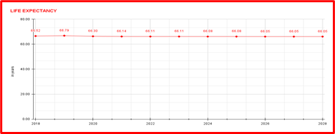
Figure 1. Life Expectancy of Population (Years) Variation with Respect to Time (Years)

A growing number of machine learning (ML) tools have been employed to deal with BMI limitations [5]. In sectors such as e-commerce, ML is useful because it can uncover patterns hidden in large datasets and offer tailored recommendations based on user activity. Autonomous antivirus software is one example of how ML can self-learn and filter new threats with no constant human supervision [6]. The efficacy of ML in the healthcare industry is apparent as it provides versatile management of diverse patient data in dynamic environments involving complex, multi-dimensional information [5].

Support and confidence are the two main metrics used to assess the power of association rules [7]. Support quantifies the frequency with which a particular rule shows up in the database throughout mining, whereas confidence measures the frequency at which a rule turns out to be accurate in practical scenarios. When a frequently occurring rule may lead to fewer general occurrences but still indicates an important connection within the collected data, this is an example of strong support but low confidence [7]. The goal of ML, a branch of artificial intelligence, is to free computers from the need of human programming to learn particular tasks [6, 8, 9].

1.1. Machine Learning (ML) Algorithms

1.1.1. Decision Tree. Decision tree is a non-parametric, supervised, learning technique with a hierarchical tree structure made up of root, branches, internal, and leaf nodes. It is used for regression as well as classification [6].

1.1.2. K-Nearest Neighbor. In order to classify or predict data, the k-nearest neighbor algorithm, also known as KNN or k-NN, groups individual data points according to their proximity. It is a non-parametric, supervised, learning classifier [6].

1.1.3. Support Vector Machine. In machine learning, support vector machines (SVMs) are supervised learning algorithms that handle tasks such as classification and regression [6]. SVMs divide a data set into two groups and are especially useful in solving binary classification problems.

Research from around the world, including from China as well as the US, shows a connection between the use of cars and obesity rates. High car usage communities frequently have higher obesity rates. Walking, cycling, and using other forms of alternative transportation for commuting may lower the risk of being overweight or obese, according to preliminary research conducted in southern Sweden. To confirm this link and guide transportation policies that support public health, more research is required [10]. Active transportation to school has the potential to improve health, although there is conflicting evidence about how it affects young people's weight outcomes.

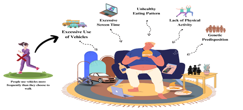
Figure 2. Social and Behavioral Factors Causing Obesity

Since exercise burns calories and improves general health and wellbeing, it is essential for managing obesity. Frequent physical activity, such as jogging, walking, and running, lowers the risk of obesity and promotes weight control, as shown in Figure 2.

2. METHOD

2.1. Association Rules

A pattern (a set of items, subsequences, substructures) that occurs frequently in a data set in association rule mining. It involves identifying inherent regularities in the data, such as the common use of personal transport among obese people or the correlation between sedentary lifestyle and high obesity rates. This technique aims to find all the rules with minimum support and confidence. In this regard, support is the probability of the transaction, while confidence is the conditional probability of the transaction.

2.2. Mining Association Rules

Mining association rules can be reduced to mining frequent items. Association rule mining is a two-step process.

1. Find all frequent items as determined by minimum support.
2. Generate strong association rules that satisfy minimum support and minimum confidence.

Support = (Frequency (X,Y))/N (1)

Confidence = (Frequency (X,Y))/(Frequency (X)) (2)

Support indicates how frequently an itemset appears in the dataset, whereas confidence indicates how often the rule is true. High support value (80%) is used to get maximum itemsets in the data set and low confidence value (25%) is used to determine maximum and multiple associations among items.

2.3 Decision Trees (DT)

Creating a model to predict a numerical variable using a set of distinct variables is the goal of this algorithm which is characterized by recursive partitioning. Nodes for decision-making and leaves make up trees. When constructing DT regression, standard variation reduction is typically taken into account when dividing a node into multiple branches, as shown in Figure 3. The initial choice of node to be split based on the most significant independent variable is the root node [11]. The parameter with the lowest sum of summed estimate (SSE) of mistakes is taken into consideration as the decision node. Moreover, nodes are separated once more. The outcomes of the chosen variable are used to partition the dataset. When a predetermined termination criterion is met, the process is said to have ended. The final nodes, referred to as depart nodes, forecast the dependent variable. This number is in line with the average of the values related to leaves [8].

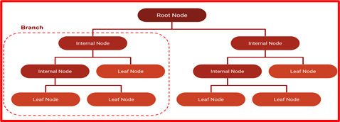
Figure 3. ML-based Algorithms

The divide-and-conquer approach of DT learning uses greedy search to find the best split points inside a tree. Recursive top-down splitting is used in this process until records are assigned particular class labels. The complexities of this technique determine how homogeneous the classified data points are; smaller trees have an easier time producing pure leaf nodes. On the other hand, data fragmentation may cause overfitting in larger trees [8]. DT, therefore, favor tiny trees, which is in line with Occam's razor’s parsimony principle which states that "entities should not be multiplied beyond necessity."

 Put another way, DTs should only add complexity when absolutely necessary because, most of the time, the simplest explanation works best. Pruning is a common technique used to minimize complexity and prevent overfitting; it involves removing branches that split on features that are not very important. Cross-validation can then be used to assess how well the model fits the data. Using the random forest (RF) technique to create an ensemble of DTs is another method to keep them correct. This classifier produces predictions that are more accurate, especially when trees have no correlation with one another [8].

The primary problem that emerges while constructing a DT is figuring out which attribute is ideal for the base node and its child nodes. In order to address these issues, a method known as attribute selection measure or ASM has been developed. It can quickly choose the ideal attribute for nodes using this measurement. For ASM, there are two widely used methods, namely knowledge acquisition and  Gini index [8].

The calculation of modifications in entropy following the attribute-based dataset segmentation is known as information gain. It determines the amount of knowledge a feature gives about a class. It divides nodes and creates the tree based on the information gain value. A node or attribute with the largest data gain is split first in a DT algorithm [11] which always seeks to maximize the amount of information gain. It can be computed using equation 3.

Information Gain= Entropy (S)-[(Weighted Avg) x Entropy (Each Feature)] (3)

A metric used to quantify the impurity of a given characteristic is called entropy. It describes the unpredictability in the data, as shown by equation 4. One way to calculate entropy is as follows,

Entropy (S) = -∑^c_(i=1)p_i log₂ P_i (4)

When building a tree using the classification and regression tree (CART) algorithm, the Gini index acts as a measure of purity or impurity. It is better to choose an attribute with a low Gini index over one with a high index. The CART algorithm only produces binary splits and it does so by utilizing the Gini index. The following equation 5 can be used to calculate the Gini index,

Gini Index= 1- ∑^c_(i=1)(p_i )² (5)

where p is probability and c is the number of classes

2.4. K-Nearest Neighbor (KNN)

Although this algorithm can also be used to solve regression problems, the KNN approach is typically used to solve classification difficulties. The concept of this algorithm is straightforward. It determines the distance between a data point and the training dataset points in order to choose the K closest ones and calculate their average as prediction, given a measurement (Euclidean distance, Mahala Nobis distance, or others) and a k-value [6]. The weighted k-nearest neighbors (WKNN) algorithm is an enhancement of this approach. In WKNN, the prediction's computation takes the weighted arithmetic mean into account.

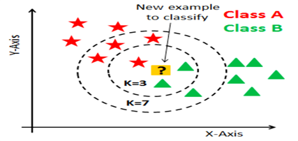
Figure 4. Graphical Representation of KNN Algorithm

2.5. KNN's Use of Distance Metrics

The KNN algorithm aids in locating the groups or closest points to a query point. However, it requires a measure to identify the closest points or groups for a given query point. Then, it employs the following distance measurements for this purpose.

Euclidean Distance is the cartesian distance between two locations in the plane or hyperplane. Another way to define Euclidean distance is to describe it as the length of the straight line connecting the two points under investigation. This metric aids in the computation of the net displacement that an object undergoes between its two states.

Since KNN is an instance-based learning algorithm, it requires all training samples to be retained in order to classify data [12]. Each test sample is compared to its K neighboring samples used as training during classification. Neighbors are typically defined using the Euclidean distance metric, while the class label prediction is generated based on a majority vote among neighboring samples.

There are differences in sample numbers for various classes due to the non-uniform distribution of data. During classification, the variable K in KNN is usually a fixed value which may lead to biases between classes. The value of K is important because a small value could cause model instability and a large value could lead to overfitting. Although cross-validation is a popular technique for figuring out K, it might not always be possible, particularly in situations like online classification [13].

When the object's total distance traveled is more important than its displacement then Manhattan distance metric can be used, as shown by equation 6. The total variation between the point coordinates in n dimensions is added together to determine this measure.

Distance= ∑ⁿ_(i=1)|p_i-q_i | (6)

Equation 7 shows the Minkowski distance,

Distance = (∑ⁿ_(i=1)|x_i-y_i |^p )^1/p (7)

where p is the degree of the dimensions of the data set. It can be 1,2,3…

2.6 Support Vector Machine (SVM)

 A supervised learning algorithm that can be used for regression or classification tasks is support vector machines (SVMs), more specifially support vector regression (SVR). SVMs maximize the distance between different output values or classes by locating a hyperplane in a high-dimensional space. As functions that gauge the resemblance between input vectors, kernels are essential to SVR. Non-linear kernels are more complex and are able to capture intricate patterns in the data, whereas linear kernels only involve an easy dot product. The characteristics of the data and task complexity determine which kernel is the best [14].

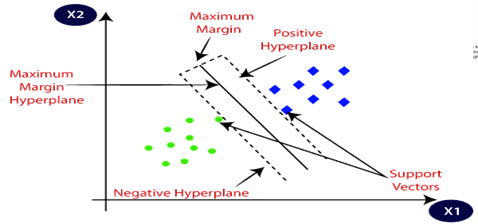
Figure 5 Graphical Representation of SVM

SVR includes a number of hyper parameters that let the users adjust the model's behavior. The C parameter, for example, controls how ‘sensitive loss’ and ‘insensitive loss’ are traded off. A smaller C value allows the model to be more forgiving of larger errors, whereas a greater C value emphasizes reducing insensitive loss [14].

The success rate of the SVR model is evaluated using common ML techniques.  The data is divided into sets for training and testing, with the former being used for fitting the model and the latter for assessment. The difference between the expected and actual output values can then be measured using statistics such as mean squared error (MSE) and mean absolute error (MAE) [14].

Mean absolute error or MAE is used to gauge how closely predictions match actual results [15]. It is calculated using equation 8.

MAE=1/n ∑ⁿ_(i=1)|y_i-(y_i) ̃| (8)

The root squared of the mean square error or MSE is the definition of an estimator with regard to the calculated parameter θ' and it can be calculated by using equation 9 [15].

RMSE=∑_(i=1)ⁿ(yi-yi ̃ /_n)² (9)

This study aims to integrate the SVM learning data into the KNN classifier. The results are compared with traditional KNN and SVM to illustrate the classification performance. The traditional SVM algorithm, as shown in equation 10, is used to identify the SVs for each class after all training points have been mapped onto the space of vectors.

D_kj=∑ⁿ_(k=1)^l√((∑_(i=1) ).(x_k )- ∑^(j=1)m_ij)² (10)

Equation 11 is used for the calculation of average distance.

aver D_k=(∑^m_(jk=1).)/m (11)

Equation 12 is used for the computation of the shortest average.

D=kmin(aver D_k ) (12)

In order to make it simple to classify fresh data points in the future, the SVM approach seeks to identify the optimal line or decision boundary that can divide n-dimensional space into classes. The optimal decision boundary is referred to as a hyperplane. SVM selects the extreme vectors and points to aid in its creation [14].

2.7 Evaluation Parameters

The formula in equation 13 is used to calculate accuracy which is the percentage of right predictions.

Accuracy=(TP+TN)/(TP+TN+FP+FN) (13)

For the computation of sensitivity and specificity, equation 14 and 15 can be used, respectively [16].

Sensitivity=TP/(TP+FN) (14)

Specificity=TN/(TN+FP) (15)

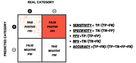
Figure 6. Confusion Matrix Representing the Relationship between Actual Classes and Predicted Classes

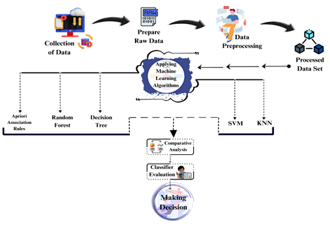
Figure 7. Block Diagram of the Proposed Methodology

3. RESULTS

3.1 Data Set

The data set was based on the daily routine and physical condition of the volunteers. The data was collected from open source UCI library. It consisted of 2111 samples with 17 features, having diffirent data types. Further, 77% of the data was generated synthetically using the Weka tool and the SMOTE filter, while the remaining 23% was collected directly from users through a web platform. There were some missing values which are replaced by mean values using rapidminer software. Then, the data set was normalized and divided into 5 categories, namely basic information, family history, eating habits, physical conditions, and harmful behavior. Figure 8 depcits the data and its classification.

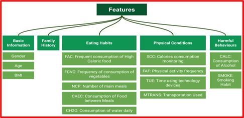
Figure 8. Data Set and its Divisions

In the training of the data set, three models based on Decision Tree, KNN, SVM. Then, data visualization was performed via Boxplot and Histogram. The age and height attributes were dropped and checked performance and then tried on all other attributes. As shown in Figure 9, the average index is very different between the use of public transportation, automobile, motor bike, and walking. Also, Figure 10 shows that although there is a lot of difference in the distribution of public and private transportation via automobiles; still, there is no big difference in the variance among them.

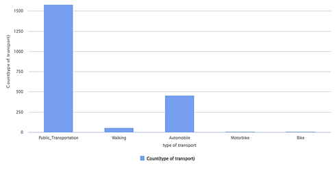
Figure 9. Distribution of Transportation Use

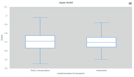
Figure 10. Box Plot Predicting the Type of Transport Used

Table 1. List of Parameters and their Associated Values

3.2 Association Rules

The parameters used for association rules are given in Table 1. On the basis of these parameters, strong association rules are given in Table 2.

Table 2. Association Rules with their Support and Confidence Values

Rule No. 1 indicates that 28% (support) of the premises (given in table-2 is maximum value and the possibility of obesity recurrence is 84% (confidence). Rule No. 2 indicates that 24% (support) of the second premises is the maximim and the possibility of obesity recurrence is 84% (confidence). Rule No. 3 indicates that 25% (support) of third premises is the highest and the possibility of obesity recurrence is 86% (confidence).

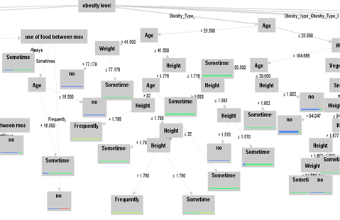
Figure 11. Decision Tree with Sub Nodes

3.3 Decision Tree (DT) Classifier

Random forest-based DT was applied on the data set, with the use of transport as the label attribute,a tree has been obtained, Figure 11 depicts a branch of the tree. The figure 11 shows that obesity is main root of tree, while its branches are divided into sublevels of obesity. Further subnodes  consist of other features.

Figure 12 depicts the confusion matrix of DT which represents predicted classes versus actual classes. It gives the overall accuracy of 90.36% and also has  find a  recall factor based on the sensitivity and specify of the confusion matrix (98.73%). The decision tells us about the people who use public transportation. It shows that the distribution of obesity among these people is more common. Most people who like to walk are able to maintain a normal body weight.

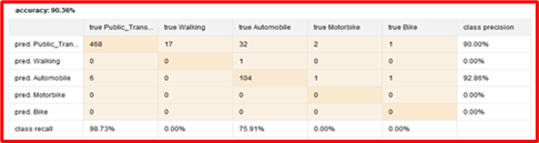
Figure 12. Confusion Matrix of DT

3.4 K-Nearest Neighbor Classifier

Several experiments for K fold parameters, from k1 to k=15, were conducted. The best performance was achieved at k9 in the calculation of KNN algorithms. The 10-fold cross-validation method was used to carry out the validation process. The data set was divided into ratios of 70% for training and 30% for testing.

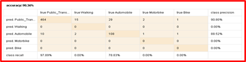
Figure 13. Confusion Matrix of KNN

3.5 Support Vector Machine (SVM)

SVM has several kernels including linear, gaussian, polynomial, and sigmoid kernels. SVM with a linear kernel was applied. As the data set has the highest distribution among features, another kernel would be produce with overfitting. In linear kernel SVM, an accuracy of 86.77% and recall factor of 97.31% was obtained. Figure 15 shows the result of SVM with scattered graph. It shows that most scattered points are of public transport and automobiles, while very few points are of walking and bike riding. Also, it can be seen that all features increase along the x-axis, which indicates that these are highly correlated with each other.

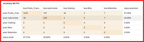
Figure 14. Confusion Matrix of SVM

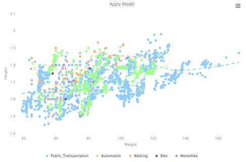
Figure 15. Scattered Graph of SVM Results

3.6 Comparative Analysis

Table 3 shows the accuracy and recall factor of all proposed ML algorithms. It shows the highest accuracy of 90.36% with a recall factor value of 98.73% for DT with random forest technique.

Table 3. Accuracy, Recall Factor, and Precession of ML Algorithms

4. DISCUSSION

Environmental factors have a major role in the global rise in obesity. These factors include high food consumption, consumption of sugary beverages, inactivity, and extensive television viewing. Social globalization constantly exposes people to cheap, enticing foods that are high in fat or calories which increases their weight.

The increasing use of cars and bicycles, even for short trips, has been identified as a significant factor. Short-distance walking has become less common and people are adopting a more sedentary lifestyle as a result of this transportation preference. The predominant mode of transportation in Pakistan is indicative of a reduction in the levels of physical activity. An additional aspect of the problem is the inadequacy of the current transportation infrastructure. Walking is not as preferred as motorized transportation [4]. The problem is made worse by an ineffective urban design and an infrastructure that is non-pedestrian-friendly.

The complex web of factors contributing to weight gain need correlations and explanations, especially for complex interactions between transportation habits and the rising rates of obesity [3, 17]. For this purpose, ML algorithms such as KNN, SVM, and DT were applied, although on the basis of strong association rules about the use of transport. DT classified the instances with high accuracy and recall factor. This algorithm proved to be more accurate for this data set because of the strong correlation between all attributes of obesity. To confirm this link and guide transportation policies that support public health, more research is needed. Active transportation to school has the potential to improve health, although there is conflicting evidence about how it affects young people's weight outcomes.

4.1. Conclusion

Overweight and obesity are related to various other diseases. The prevalence of obesity has increased considerably and it is estimated that by 2030, it will be around 50%. In this study, the aim was to predict the major cause of obesity in Pakistan. For this purpose, in-depth research was conducted by using various ML techniques including KNN classifier, SVM, and DT classifier on the dataset collected from open source UCI library. The analysis showed a strong relationship between the use of personal transport due to the adoption of a sedentary lifestyle causing an increase in the obesity level. Furthermore, 10-fold cross-validation was used and hyperparameters of tested models were optimized. The results showed that the DT algorithm obtained the best results with 90.36% accuracy. Future research should validate the results with other relevant groups.Furthermore, differences in the prediction of obesity status at district, city, and province level in Pakistan should be evaluated with regional disaggregation.

Conflict of Interest

The author of the manuscript has no financial or non-financial conflict of interest in the subject matter or materials discussed in this manuscript.

Data Availability Statement

The data associated with this study will be provided by the corresponding author upon request.

Bibliography

- World Helath Organizarion. Obesity and overweight. WHO Web site. https://www.who.int/news-room/fact-sheets/detail/obesity-and-overweight. Updated March 1, 2024. Accessed April 2, 2024.
- Laar RA, Shi S, Ashraf MA, Khan MN, Bibi J, Liu Y. Impact of physical activity on challenging obesity in Pakistan: a knowledge, attitude, and practice (KAP) study. Int J Environ Res Public Health. 2020;17(21):e7802. https://doi.org/10.3390/ijerph17217802
- Randhawa FA, Mahmud G, Rasheed S, Asad A. Obesity in Pakistan - a new epidemic. Rawal Med J. 2021;46(2):446–449.
- Tanveer M, Hohmann A, Roy N, Zeba A, Tanveer U, Siener M. The current prevalence of underweight, overweight, and obesity associated with demographic factors among Pakistan school-aged children and adolescents—an empirical cross-sectional study. Int J Environ Res Public Health. 2022;19(18):e11619. https://doi.org/10.3390/ijerph191811619
- Rathore DK, Mannepalli PK. A review of machine learning techniques and applications for health care. Paper presented at: International Conference on Advances in Technology, Management and Education (ICATME); januayr 8–9, 2021, Bhopal, India. https://doi.org/10.1109/icatme50232.2021.9732761
- Wiyono S, Wibowo DS, Hidayatullah MF, Dairoh D. Comparative study of KNN, SVM, and decision tree algorithm for student’s performance prediction. Int J Comput Sci Appl Math. 2020;6(2):50–53. https://doi.org/10.12962/j24775401.v6i2.4360
- Uddin S, Khan A, Hossain ME, Moni MA. Comparing different supervised machine learning algorithms for disease prediction. BMC Med Inform Decis Mak. 2019;19(1):e281. https://doi.org/10.1186/s12911-019-1004-8
- Méndez M, Merayo MG, Núñez M. Machine learning algorithms to forecast air quality: a survey. Artif Intell Rev. 2023;56(9):6957–6981. https://doi.org/10.1007/s10462-023-10424-4
- Sukmawati, Sirajuddin. Correlation of maternal education with parenting and child nutritional status. Indian J Public Health Res Dev. 2019;10(9):74–78. https://doi.org/10.5958/0976-5506.2019.02545.2
- Barranco-Ruiz Y, Guevara-Paz AX, Ramírez-Vélez R, Chillón P, Villa-González E. Mode of commuting to school and its association with physical activity and sedentary habits in young Ecuadorian students. Int J Environ Res Public Health. 2018;15(12):e2704. https://doi.org/10.3390/ijerph15122704
- Kingsford C, Salzberg SL. What are decision trees? Nat Biotechnol. 2008;26(9):1011–1012. https://doi.org/10.1038/nbt0908-1011
- Cover TM, Hart PE. Nearest neighbor pattern classification. IEEE Trans Inf Theory. 1967;13(1):21–27. https://doi.org/10.1109/tit.1967.1053964
- Meng Q, Cieszewski CJ, Madden M, Borders BE. K nearest neighbor method for forest inventory using remote sensing data. GIsci Remote Sens. 2007;44(2):149–165. https://doi.org/10.2747/1548-1603.44.2.149
- Noble WS. What is a support vector machine? Nat Biotechnol. 2006;24(12):1565–1567. https://doi.org/10.1038/nbt1206-1565
- kumar Y, Sahoo G. Study of parametric performance evaluation of machine learning and statistical classifiers. Intl J Info Technol Comput Sci. 2013;5(6):57–64. https://doi.org/10.5815/ijitcs.2013.06.08
- Altman DG, Bland JM. Statistics notes: diagnostic tests 1: sensitivity and specificity. BMJ. 1994;308:e1552. https://doi.org/10.1136/bmj.308.6943.1552
- Churchill SA, Koomson I, Munyanyi ME. Transport poverty and obesity: The mediating roles of social capital and physical activity. Transp Policy (Oxf). 2023;130:128–136. https://doi.org/10.1016/j.tranpol.2022.11.006