Bivariate and Multivariate Data Cloning through Non Linear Regression Models

Sajid Hussain^1*, Zafar Iqbal¹, Muhammad Mansoor², and Rashid Ahmed¹

¹Department of Statistics, The Islamia University of Bahawalpur, Pakistan

²Department of Statistics, Government S. E. College, Bahawalpur, Pakistan

* Corresponding Author: [email protected]

ABSTRACT

Nonlinear regression analysis holds significant popularity in mathematical, engineering, and social science domains. Disciplines like financial matters, biology, and natural chemistry have broadly utilized nonlinear regression models (NLRMs). Cloned datasets have their own importance in such areas which provide the same fit of bivariate and multivariate nonlinear regression models for the actual datasets. This article presents a sequence of cloned datasets that give exactly the same fit of bivariate and multivariate nonlinear regression models.

Keywords: cloned data, nonlinear regression model, fictitious datasets, data visualization.

1. INTRODUCTION

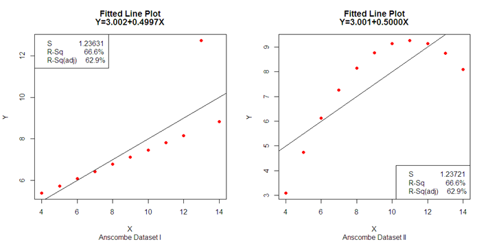
If genuine information is private and cannot be shown, a matching or alternative set of data is required which provide same summary statistics as of the actual data. Cloned data refers to the alternative or matching set of data through mathematical techniques that allow rapid provisioning in testing and developments. Data cloning has its own significance as an alternative method for protecting confidential information and database. Table 1 shows four fictitious distinct cloned datasets (CDSs) created by Anscombe [1] to demonstrate the significance of graphs in statistical analysis. The summary statistics (mean, standard deviation, and correlation) as well as the parameter estimates of the fitted regression equation R² and estimated standard deviation of residuals are identical across these four distinct CDSs, however, they were vastly different scatter plots as shown in Figure 1. Dataset I was strongly linear with a single outlier and II appears to follow a parabolic distribution, whereas dataset III appears to adhere to a noisy linear regression model (LRM), and dataset IV appears to follow a vertical line with the regression thrown off by a single outlier. Datesets in Table 1 are significant and frequently used to show how important visible methods are. These datasets were also known for their significant use in education. However, the method used to create the datasets was not explained in [1]. A genetic algorithm-based approach was proposed by Chatterjee and Firat [2], who generated 1,000 random datasets with comparable summary statistics and graphics for the basic datasets. Govindaraju and Haslett [3] devised a method for producing datasets by regressing the response on the covariate in the direction of their unconditional sample means, while maintaining identical LRM estimates. As a result, the variability in the response and the covariate decreased in each subsequent cloned dataset. Haslett and Govindaraju's [4] method for creating matched datasets was extended to include a multiple linear regression model, ensuring that the matched datasets have an identical fit to the original data. The idea of data-cloning emerged from both biostatistics [5, 6] and financial time series [7].

Cloning for maximum likelihood estimation using Bayesian software was achieved by the simple device of replicating the original data many times [6]. Fung et al. [8] expressed that the creation of CDSs to anonymize sensitive data was another application for datasets with the same statistical properties, as discussed in [3]. In this instance, it is critical that individual data points were altered, while the data's overall structure remained unchanged.

Haslett and Govindaraju [9] described a straightforward approach for modifying LRM data, while still obtaining the same fitted regression parameters. Ponciano et al. [10] showed how structural parameter non-identifiability can be diagnosed with Data Cloning (DC) and distinguished from other parameter estimability issues, such as when parameters are structurally identifiable but not estimable in a given data set or when they are identifiable and weakly estimable. Bayesian phylogenetics software can be used to diagnose non-identifiability with the DC approach. Additionally, it was demonstrated that DC can be used to examine and eliminate the influence of priors, particularly when prior elicitation was difficult. Finally, DC can be used to investigate at least two significant statistical issues when applied to phylogenetic inference, developing effective sampling strategies for computationally expensive posterior densities, and evaluating the identifiability of discrete parameters, such as the tree's topology.

Data confidentiality is one of the designed goals of tunable encrypted deduplication, see Amvrosiadis and Bhadkamkar [11]. Additionally, it reduced the risk of data leakage brought by frequency analysis. Furthermore, it was identified that better ways of seeing and exploring data lead to better insights. The "Datasaurus" Cairo dataset was created by Alberto Cairo [12]. This, like Anscombe's Quartet, emphasized the significance of data visualization, despite the dataset's normal summary statistics, the plot it produced depicted a dinosaur. They started with the datasaurus and created additional datasets with the same summary statistics. Additionally, Cairo's Datasaurus data visualization prohibited to solely rely on the summary statistics of the used data.

Resultantly, according to [2], datasets should be as graphically distinct as possible. With different standard deviations but identical means and LRM estimates, [3, 4, 9] data are intended to be graphically comparable. Matejka and Fitzmaurice [13] developed a novel method for creating datasets, which are identical across a variety of statistical properties but visually distinct during the data exploration. To address the primary empirical facts of financial time series, numerous complex parametric stochastic volatility models were proposed in the subsequent literature. The models that Mao et al. [14, 15] proposed incorporated a broader asymmetric volatility function.

Hussain et al. [16] used a simple procedure to clone data for nonlinear regression models having linearizable or nonlinearize regression functions, such as aX^b, ab^X, ae^bX, k ks^X k+ab^X,k/(1+bc^X) A[aX₂^(-b)+(1-a)X₁^(-b)]^(-1/b). They found that cloned data generated by linearizable or non-linearizable estimable functions of parameters have unchanged estimates. The procedure increased the sample size of cloned data without changing the parameters estimates, which was for n original sample points (x, y). This generated n² observations by adding [a_i: i = 1, 2, …, n] to the data points y over ∑_i a_i = 0. Due to increased sample size, cloned estimates showed smaller standard errors as compared to the original standard errors. This procedure used by [16] was sufficient for the first iteration because in the next iterations, it became tedious work. This procedure was useful for modeling but not for confidentialising or encrypting data, as in the design matrix variables remained unchanged. In this case, the term "confidentializing" referred to making the values of particular variables certain for particular people that cannot be deduced from the data. Our goal in this article is to create datasets with the same fit for nonlinear linear regression models (NLRMs). [3, 4] methods were used to generate these cloned data sets. To get around the problem in [16], nonlinear regression models with linearizeable regression functions were the prime focus of this article.

Table 1. Anscombe's CDSs with Pairs (x, y₁), (x, y₂), (x, y₃) and (x₄, y₄)

Figure 1. Scatter Plots of Anscombe's Datasets with Matched Simple Regression Models

2. THE NONLINEAR REGRESSION MODEL

2.1. The Regression Model (RM)

The Regression Model (RM) talks about the relationship between a response variable and one or more covariates X^(j). The general model is:

Y_i=H(X_i⁽¹⁾,X_i⁽²⁾,…,X_i^(m);A₁,A₂,…,A_p)+E_i

Here, H is a suitable function that relies on the covariates X_i⁽¹⁾,X_i⁽²⁾,…,X_i^(m) and parameters A₁,A₂,…,A_p. The unstructured deviations from H are defined by means of random errors (REs) E_i~N (0,σ² ).

2.2. The Linear Regression Model

In multiple LRM (MLRM), function H are characterized as linear in the parameters.

(X_i⁽¹⁾,X_i⁽²⁾,…,X_i^(m);A₁,A₂,…,A_p)=A₁ X ̃_i⁽¹⁾+A₂ X ̃_i⁽²⁾+ ⋯ +A_p X ̃_i^(m)

where X ̃_i^(j) can be arbitrary functions of the original covariates X_i^(j).

2.3. The Nonlinear Regression Model

In NLRM, function is regarded in such a way that it can't be written as linear in parameters. In case, there are infinite ways to explain the deterministic part of the model.

2.4. Linearizable Regression Functions (LRFs)

In NLRMs, functions can be linearized by the transformation of the variable of interest and the explanatory variables. Therefore, the regression is named as function which is linearizable if it can be converted into a function linear in the parameters.

2.5. A Few Examples of Nonlinear Regression Functions

1. H(X_i ;A₁ ,A₂)=A₁ X_i^(A₂)

2. H(X_i;A₁ ,A₂)=A₁ A₂^(X_i)

3. H(X_i;A₁ ,A₂)=A₁ e^{(A₂ X_i)}

4. H(X_i⁽¹⁾ ,X_i⁽²⁾ ;A₁,A₂,A₃= A₁ (X_i^{(1)(A₂)(A₂) (X_i(2)(A₃)}

2.6. Linearizable Regression Function Model

A LRM with the LRF in the referred example is based on the model given below:

ln⁡(Y_i)=B₁+B₂ X ̃_i⁽¹⁾+B₃ X ̃_i⁽²⁾+E_i; X ̃_i⁽¹⁾=ln⁡(X_i⁽¹⁾,X ̃_i⁽²⁾=ln⁡(X_i⁽²⁾

Where, E_i follows the normal distribution. This model was back-converted and for this reason, the following equation was obtained:

Y_i=A₁ (X_i⁽¹⁾) ^(A₂)) (X_i^{(2) (A₃)} E ̃_i; E ̃_i= exp⁡(E_i),i=1,2,…,n

The errors E ̃_i follows lognormal distributed and contributed multiplicatively. The assumptions about the random deviations were accordingly now appreciably distinct for a model, which was primarily based on:

Y_i=A₁(X_i^(1)(A₂)(X_i^(2)(A₃)+E_i^*

with random deviations that follows normal distribution and contributed additively.

3. DATA CLONING BY USING REGRESSING Y ON X AND X ON Y

Assuming n paired observations of X and Y say (x_i,y_i) i=1,2,⋯,n. The following procedure from [3] would generate a sequence of CDSs by obtaining the same fitted NLRM equations.

3.1. Procedure for Bivariate Nonlinear Regression Model

The simple NLRM (a geometric or power curve) Y=AX^B was linearizable due to logarithmic transformation as Y ̃=a+BX ̃ where Y ̃= ln⁡(Y),X ̃= ln(X), a=ln⁡(A), and A=exp⁡(a). The inverse nonlinear regression model (INLRM) of Y=AX^Bi is =(Y/C)^(1/D), which was also linearizable as X ̃=c+dY ̃ where where d=1/D,D=1/d ,c=-(ln⁡(C)/D ,C=exp⁡(-c/d).

1. First fit regression Y ̃on X, namely Y ̃₁=a+BX. Also fit inverse regression (IR) X on Y namely X ̃₁=c+dY ̃ .
2. The regression of Y ̃₁ on X ̃₁ would be Y ̃₂=a+BX ̃₁, preserving same parameter estimates. Likewise, X ̃₂=c+dY ̃ ̃₁. Note that S _{(Y ̃1)}² < S _{(Y ̃2)}² and S _{(X ̃1)}² < S _{(X ̃2)}²
3. The above method can be iterated with Y ̃₂ and X ̃₂ as done in step 1 to gain cloning sets of data having the identical linearizable regression equation (LRE). Again S _{(Y ̃1)}² < S _{(Y ̃2)}² < S_(Y)² and S _{(X ̃1)}² < S _{(X ̃2)}² < S_(X)²
4. If preferred, transform back for CDSs, having same coefficients of NLRM. It was noted that variability in Y and X of the cloned datasets fluctuated after every iteration (see Table 2).

Example 1. Consider the variables X= (0.5, 1.5, 2.5, 5.0, 10.0)^T and Y= (3.4, 7.0, 12.8, 29.8, 68.2)^T, resulting in the nonlinear regression fit Y ̂=5.709057X^1.01876 (3.1)

Steps 1-4 given above would yield the CDSs proven in Table 2. with exactly the same equation of fitted NLRM as in (Eq. 3.1).

Table 2. Cloned Data Sets Having the same Non Linear Regression Fit Y=AX^Bt

3.2. Procedure for Bivariate Nonlinear Regression Model Y=AB^X

A simple nonlinear regression model (an exponential curve) Y=AB^X was linearizable due to logarithmic transformation as Y ̃=a+bX where Y ̃=ln⁡(Y),a=ln⁡(A) ,A=exp⁡(a), b=ln⁡(B), and B=exp⁡(b). The inverse nonlinear regression model of Y=AB^X was which was X=ln(Y/C)^(1/(ln⁡(D) also linearizable, as X=c+dY ̃where where d=1/(ln⁡(D,D= exp⁡(1/d) ,c=-(ln⁡(C)/(ln⁡(D),C=exp⁡(-c/d)..

1. First fit the regression of Y ̃on X specifically Y ̃₁=a+bX. Also, fit the IR of X on Y particularly X̃₁=c+dY.
2. The regression of Y ̃̃₁ on X̃₁1 would be Y ̃̃₂=a+bX̃₁, maintaing the identical parameter estimates. Similarly, X̃₂=c+dY ̃̃₁. Note that S _{(Y ̃1)}² < S _{(Y ̃2)}² and S _{(X ̃1)}² < S _{(X ̃2)}²
3. The above prcedure can be iterated with Y ̃sub>2 and X₂ as in step 1 to obtain CDSs having the same LRE. S _{(Y ̃1)}² < S _{(Y ̃2)}² < S_(Y)² and S _{(X ̃1)}² < S _{(X ̃2)}² < S_(X)²
4. If preferred, convert back to produce a sequence of CDSs, all with the same NLRM coefficients. Therefore, it was observed that variability in Y of the cloned datasets fluctuated after each and every generation (see Table 3).

Example 2. Consider the variables X= (0, 1, 2, 3, 4, 5, 6, 7, 8)^T and Y= (0.75, 1.20, 1.75, 2.50, 3.45, 4.70, 6.20, 8.25, 11.50)^T and resulting in the nonlinear regression fit

Y ̂=(0.8573324)(1.392474)^X (3.2)

Steps 1-4 described above would generate the CDSs presented by Table 3 having exactly same NLRM fitted equation as in (Eq. 3.2).

Table 3. Cloned Data Sets Having the same Nonlinear Regression Fit Y=AB^X

3.3. Procedure for Bivariate Nonlinear Regression Model Y=Ae^BX

The simple nonlinear regression model (an exponential curve) Y=Ae^BX was linearizable due to logarithmic transformation as Y ̃=a+BX where Y ̃=ln⁡(Y),a=ln⁡(A), and A=exp⁡(a). The inverse nonlinear regression model of Y=Ae^BX was X=ln(Y/C)^(1/D) , which was also linearizable as X=c+d(Y ) ̃where d=1/D,D=1/d, c=-(ln⁡(C))/D, C=exp⁡(-c/d).

1. First fit simple LRM of Y ̃ on X representing Y ₁=a+BX. Also, fit the simple inverse LRM of X on Y ̃describing X₁=c+dY ̃as .
2. The regression of Y ̃₁ on X₁  would be Y ̃₂=a+BX₁, saving the alike parameter estimates. In the same way, X₂=c+dY ̃₁. Note that S _{(Y ̃1)}² < S _{(Y ̃2)}² and S _{(X ̃1)}² < S _{(X ̃2)}²
3. The approach used above can be iterated with Y ̃₂ and X₂ as in step 1 to get CDSs with the same LRE. Again S _{(Y ̃1)}² < S _{(Y ̃2)}² < S_(Y)² and S _{(X ̃1)}² < S _{(X ̃2)}² < S_(X)²
4. If preferred, transform back to get a sequence of CDSs, all with the same NLRM coefficients. It was observed that variability in Y of the cloned datasets fluctuate after every iteration (see Table 4).

Example 3. Consider the variables X= (0.5, 0.8, 1.4, 2.0, 2.5)^T and Y= (9.1, 8.5, 7.5, 6.7, 6.1)^T and resulting in the nonlinear regression fit Fit Y=AB^X

Y ̂=9.989049e^{(-0.1991399X)} (3.3)

Here, the CDSs would be yielded as shown in Table 4, using steps 1-4 discussed earlier, to produce same equation of fitted NLRM as given in (Eq. 3.3).

Table 4.  Cloned Data Sets Having the Same Nonlinear Regression Fit Y=Ae^BX

We have generated the cloned data sets for following nonlinear regression models models Y=1/(A+BX), Y=A+B/(1+X), Y=A+B√X, Y=AX²+BX and Y=A+BX+CX² by using the procedure given by [3] and presented, respectively in Table 5-9.

Table 5. Cloned Data Sets Having the Same Non Linear Regression Fit Y=1/(A+BX);A=82.97359,B=-36.58871

Table 6. Cloned Data Sets Having the Same Non Linear Regression Fit Y=A+B/(1+X) ;A=0.086506,B=-0.091625

Table 7. Cloned Data Sets Having the Same Non Linear Regression Fit Y=A+B√X;A=-2.341445,B=3.011197

Table 8. Cloned Data Sets Having the Same Non Linear Regression Fit =AX²+BX;A=0.4,B=5.0

Table 9. Cloned Data Sets Having the Same Non Linear Regression Fit =A+BX+CX²;A=1.0,B=-0.20,C=0.20

4. CLONING FOR MULTIPLE NONLINEAR REGRESSION MODEL Y=A₀ (X_i^(1)(A₁)X_i^(2)(A₂) VIA PIVOTS

In accordance with [4], the current approach was extended to a structure of an arbitrary error covariance after discussing data that were independent and identically distributed (iid). Let us give the multiple NLRM in (Eq. 4.1).

Y_i=A₀(X_i)^(1)A₁(X_i)^A₂ E_i (4.1)

Where Y is response vector, X=(X ⁽¹⁾:X⁽²⁾ is the covariate data matrix (CDM), α=(A₀,A₁,A₂)^Tis parameters vector, and random error vector.

Eq. 4.1 is linearizable due to logarithmic transfomation, then Eq. 4.1 becomes ln⁡(Y_i)=ln⁡(A₀)+A₁ln⁡(X_i⁽¹⁾+A₂ln⁡(X_i⁽²⁾+E. Setting Y ̃=ln⁡(Y_i), X ̃⁽¹⁾=ln⁡(X_i⁽¹⁾, X ⁽²⁾ =ln⁡(X_i⁽²⁾, E ̃=ln⁡(E_i), B₀=ln⁡(A₀), B₁=A₁ and B₂=A₂ we get

Y ̃=B₀+B₁ X ̃⁽¹⁾+B₂ X⁽²⁾+E ̃ (4.2)

where Y is response vector, X ̃=(X ̃⁽¹⁾):X ⁽²⁾ is CDM, β=(B₀,B₁,B₂)^T is unknown parameters vector and E errors vector. When matrix X of rank full as column, estimates of β by ordinary least square (OLS) is b=(X^tX)^(-1) X^tY fitted multiple LRE is

Y ̃₁=b₀+b₁ X ̃⁽¹⁾+b₂ X ̃⁽²⁾ (4.3)

These consequences follow whether or not, Y ̃, X ⁽¹⁾and X ̃⁽²⁾ are mean corrected (MCtD), as here. Due to the MCtD, (Eq. 4.3) , which can be written as:

y ̂=b₁ x₁+b₂ x₂ (4.4)

where, y ̂=Y ̃-Y ̃ ̅, x₁=X ̃(1)-X ̃ ̅⁽¹⁾ and x₂=X ̃⁽²⁾-X ̃ ̅⁽²⁾.(In order to avoid any loss of generality, the column of 1 in design matrix X is eliminated following the imply MCtD because it transforms into a column of zeros).

The identified problem here was to create a new response variable vector, Y_clone, and a new covariate data matrix, X_clone. This can be easily accomplished by transposing back to Y ̃_clone and X ̃_clone, such that b=(X ̃_clone^T X ̃_clone)^(-1) X ̃_clone^T Y ̃_clone

Alternatively, multivariate CDSs to be required (Y_clone,X_clone⁽¹⁾,X_clone⁽²⁾ which produced the same multiple NLRM equation as the original dataset Y,X ⁽¹⁾,X⁽²⁾.

Returning to the case of iid, how generation of CDSs can be accomplished via manipulating any one covariate, was exhibited, say x_j, where j=1,2., using the steps below.

• Iniatially, fit multiple linearizable RM ( 4.4), using MCtD data.
• Select a covariate x₂ .
• Let y=k+b₂ x₂, where k=b₁ x₁=y ̂-b₂ x₂. To obtain the estimated values of y ̂_k and x ̂₂, perform simple RM of y_k=y-k on x₂ and inverse simple regression of x₂ on y_k.
• Regress x₁ on x₂ and obtain x ̂₁. Also, obtain x₁,2=x₁ -x₂ (x₂^t x₂)^(-1) x₂^t x₁=(I-x₂(x₂^tx₂)^(-1) x₂^t ) x₁, where I is the identity matrix.
• Form y_(k,clone)=y ̂_(k)+∑ b₍₁₎ x₁,2
• On all newly acquired x₁,2 and x ̂₍₂₎, perform multiple LREs of y_(k,clone) at the same time, where x ̂₂=y(y^ty)^(-1) y^t x₂ in which y=(1:y) is n×2. .
• If you prefer, you can add back Y ̃ ̅, X ̃ ̅^(-1), and X ̃ ̅⁽²⁾ to the cloned data or multiply all of the cloned data by the same scale factor.
• Transform back to the cloned data in step 7.
• Repeat from one to eight steps to create a series of datasets with identical NLRM coefficients. At each iteration, a different possible value of j can be chosen.

Example 4. With uncorrelated data and design matrix of full-rank, consider variables X₁, X₂ and Y in Table 9 and resulting in the multiple NLRM fit

Y ̂=1.663079X₁^0.6163121 X₂^0.2931787 (4.5)

For CDSs in Table 10, 1-9 steps specified above were used (first X₂ was used for manipulation) for which the fitted multiple NLRM equation was exactly the same as in (Eq. 4.5).

Table 10. Cloned Data Sets Having the Same Multiple Nonlinear Regression Fit Y=A₀ X₁^(A₁) X₂^(A₂)

Figure 2, represent a matrix plot of raw and cloning data in Table 10, which show the effect on X2 done by orthogonal manipulation as described in steps 1-9 of the algorithm. Bivariate relationship strength between X2,clone and Yclone is much weaker than X2 and Y. However, this is not the case with X1,clone and Yclone, because the manipulation was not done with X1.

Figure 2. Matrix Plot of raw and cloned data

5. DISCUSSION

This study showed that the parameter estimates of the original datasets discussed in this artical and their generated cloned datasets were identical. As a result, it was identified that data cloning had the potential to be used in a wide range of applications, including data encryption, visualization, and smoothing. The application of encryption was particularly intriguing because it can be used to generalize the databases even when regression modeling was not desired. In prior literature, cloned datasets were generated for linear regression models. However, it had equal importance to be generated for the nonlinear regression models. In this context, new methods can be developed for nonlinear regression models to conduct cloning for the datasets or databases.

5.1. Conclusion

CDSs have been presented for bivariate and multivariate NLRMs that have linearizable regression functions including AX^B,AB^X,Ae^BX,1/(A+BX),A+B/(1+X),A+B√X,AX²+BX,A+BX+CX² and A₀(X_i^(1)(A₁)(X_i²(A₂) with exactly the same nonlinear regression coefficients. In terms of bivariate LRFs, the response and a covariate of the CDSs collapsed to their means, which had smaller variability when compared to the original dataset..

REFERENCES

1. Anscombe FJ. Graphs in statistical analysis. Am Statistic. 1973;27(1):17–21.
2. Chatterjee S, Firat A. Generating data with identical statistics but dissimilar graphics: A follow up to the Anscombe dataset. Am Stat. 2007;61(3):248–254. https://doi.org/10.1198/000313007X220057
3. Govindaraju K, Haslett SJ. Illustration of regression towards the mean. Int J Matim Edu Sci Technol. 2008;39(4):544–550. https://doi.org/10.1080/00207390701753788
4. Haslett SJ, Govindaraju K. Cloning data: Generating datasets with exactly the same multiple linear regression fit. Aust New Zealand J Stat. 2009;51(4):499–503. https://doi.org/10.1111/j.1467-842X.2009.00560.x
5. Lele SR, Dennis B, Lutscher F. Data Cloning: Easy maximum likelihood estimation for complex ecological models using bayesian markov chian monte carlo methods. Ecol Lett. 2007;10:551–563. https://doi.org/10.1111/j.1461-0248.2007.01047.x
6. Lele SR, Nadeem K, Schmuland B. Estimability and likelihood inference for generalized linear mixed models using data cloning. J Am Stat Assoc. 2010;105:1617–1625. https://doi.org/10.1198/jasa.2010.tm09757
7. Jacquier E, Johannes M, Polson N. MCMC Maximum likelihood for latent state models. J Econom. 2007;137:615–640. https://doi.org/10.1016/j.jeconom.2005.11.017
8. Fung BCM, Wang K, Chen R, Yu PS. Privacy-preserving data publishing: A survey of recent developments. ACM Comput Surv. 2010;42(4):e14. https://doi.org/10.1145/1749603.1749605
9. Haslett SJ, Govindaraju K. Data cloning: Data visualization, smoothing, confidentiality, and encryption. J Stat Plan Infer. 2012;142:410–422. https://doi.org/10.1016/j.jspi.2011.07.020
10. Ponciano JM, Burleigh JG, Braun EL, Taper ML. Assessing parameter identifiability in phylogenetic models using data cloning. Syst Biol. 2012;61(6):955–972. https://doi.org/10.1093/sysbio/sys055
11. Amvrosiadis G, Bhadkamkar M. Identifying trends in enterprisedata protection systems. Paper presented at: USENIX Annual Technical Conference; July 8–10, 2015; Santa Clara, USA.
12. Download the Datasaurus: Never trust summary statistics alone; always visualize your data. Cairo website. http://www.thefunctionalart.com/2016/08/downloaddatasaurus-never-trust-summary.html
13. Matejka J, Fitzmaurice G. Same stats, different graphs: Generating datasets with varied appearance and identical statistics through simulated annealing. Paper presented at: Proceedings of the 2017 CHI Conference on Human Factors in Computing Systems; May 6–11, 2017; Denver Colorado, USA. https://doi.org/10.1145/3025453.3025912
14. Mao X, Ruiz E, Veiga H. Threshold stochastic volatility: Properties and forecasting. Int J Forec, 2017;33(4):1105–1123. https://doi.org/10.1016/j.ijforecast.2017.07.001
15. Mao X, Ruiz E, Veiga H, Czellar V. Asymmetric stochastic volatility models: Properties and particle filter-based simulated maximum likelihood estimation. Econom Stat. 2020;13:84–105. https://doi.org/10.1016/j.ecosta.2019.08.002
16. Hussain S, Daniyal M, Ogundokun RO, Muhammad YS, Iqbal Z, Ahmed, R. Cloning data with unchanged estimates of estimable non-linear functions of parameters. F1000Research. 2022;10:e106. https://doi.org/10.12688/f1000research.28297.2