Influence of Radiation on the Slip Flow of Hydromagnetic Fluid through a Semi-porous Channel

1. INTRODUCTION

In different research sectors, many schools of thought exist regarding the behavior of liquids traveling through semi-permeable flasks. This is useful in the medical field as it helps to purify blood in artificial kidneys [1] and oxygenate [2] blood in capillaries [3]. Kamışlı et al. [4] successfully found the channel flow of non-Newtonian fluids with wall suction or injection and solved the Navier-Stokes equation for flow in a semi-porous channel with steady, incompressible, and adhesive characteristics. Afterwards, the above research was furthered to incorporate both Newtonian and non-Newtonian fluids [5–13].

There are multiple approaches to MHD flow with respect to convection, for instance, in the study of plasma, medical sciences, and geophysics. Ziabakhsh and Domairry [14] presented the homotopy analysis method (HAM) solution of the laminar viscous flow in a semi-porous channel with a uniform magnetic field. They also attempted to solve the same problem, but with the help of HAM. Rundora and Makinde [15] studied the porous saturated medium flow of the fluid. Shekholeslami et al. [16] applied the optimal homotopy asymptotic approach to get the exact results of magnetic field effects on an adhesive motion through a semi-porous channel. Abbas et al. [17] discussed the results of the hydromagnetic flow of a second-grade fluid, which is chemically reactive, in a semi-permeable medium by using HAM.

The current research helps to find answers to all the questions about the impact of thermal radiation on the hydromagnetic Newtonian flow of fluid through a semi-porous channel. The slip condition is used on the lower wall of the channel. Linear ordinary differential equation gives the movement of the fluid and the temperature. HAM [18–20] is used to find its solution. At the end, the convergence and comparison of new results with old ones using no slip condition are presented in detail.

2. Flow Equations

Consider a channel having semi-porous boundaries filled with viscous, incompressible electricity conducting fluid, as shown in Figure 1. The fluid is injected into the channel from a wall at a distance  from the -axis, whereas external heat is applied to the wall lying along -axis. A uniform magnetic field with intensity  is taken orthogonal to the flow. The small Reynolds number assumption is utilized to abandon the impacts of the induced magnetic field.

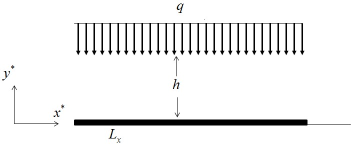
Figure 1.  Geometry of the Problem

The equations of velocity and temperature are given below.

The flow equations are stated below.

Here, u ̃ and v ̃ denote horizontal and vertical parts of the velocity and c_p, T, μ, v, ρ, ν, p, L, σ, k and q_r are the specific heat points at constant pressure, temperature of the fluid, dynamic viscosity, kinematic viscosity, density, pressure, velocity gradient, electrical conductivity, thermal conductivity, and radiative heat flux,  respectively.

The following equations give the boundary of the problem.

In the above equation, l represents slip constant, whereas l=0 indicates the absence of the slip condition.

The Rosseland approximation for radiative heat flux is used.

Here, σ^* is Stefan-Boltzman constant and k^* denotes the absorption coefficient. Since variation in temperature inside the flow is quite slight, so we can use the Taylor series of order 4 about T_∞ to get the expansion of T ⁴, where T_∞ is a linear function of T.

We get

Using eqs. (8) & (9), eq. (6) becomes

 Consider   , where N_r is a radiation parameter. So, eq. (7) becomes

To calculate U, the mean velocity, the following equation is applied

Using the dimensionless transforms,

Using eqs. (12) and (13), the dimensionless equations for continuity and momentum, eqs. (3)-(5) and energy eq. (11) yield

In the above equation, ε is the dimensionless number and is given by ε=h/L_x , where h is the distance and L_x is very small (length  of the slider in x direction), M represents the Hartmann number given by M =B₀ h√(σ/μ),  denotes the Prandtl number given by P_r⁡= (μc_p)/k, E_k  is the Eckert number given by E=U₀²/(T_h-T₀)c_p, , and R_e is the Reynolds number given by R_e=hq/v .

Using similarity transformation independent of aspect ratio ε introduced by Berman,

The continuity of eq. (14) is identically satisfied. Substituting eq. (18) in eq. (16), one can see that the quantity ∂p/∂y does not involve the longitudinal variablex . It is also observed that ∂² p/∂x² does not depend upon . A separation of variable yields the following equations,

where the symbols of primes represent the number of derivatives.

Differentiating the above eq. 19 with respect to y , we get

The respective conditions are

Here is the slip parameter given by β=l/h .

By combining eqs (17) and (18), we get

The optimal solution of eq. (22) is represented as follows:”

The respective boundaries are  

Using eq. (18) into eqs. (15) and (16), we get

Suppose in this problem is independent of the longitudinal variable , therefore, we consider

In this case, eq. (26) becomes

3. Solution Technique

Homotopy anslysis method (HAM) is applied to solve this problem. It is better than many other analytical techniques because it involves series expansion and does not depend upon large or small parameters. Further, it provides an easy way to get the best result of the problem.  

To get the output of the problem, HAM is used, as pointed out by Liao [20]. The initial guess for the given problem includes

 The following are auxiliary linear operators,

which satisfy the following properties,

where c₁,c₂,.......,c₈ are constants to determine. The equations of zeroth order deformation are given below.

with boundary conditions,

where ℏ_V,ℏ_U "and" ℏ_θ are auxiliary parameters whose values are not zero and q represents an embedding parameter with  0  q  1. Whereas, N₁,NN₁, are nonlinear operators.

For q=0 and q=1, the solutions of deformation equations of order zero are given below.

Applying Taylor's series to expand V(y,q),U(y,q)"and" θ(y,q) about q, we have

where

It is observed that the convergence of the considered problem equations (38)-(40) is based on the auxiliary parameters ℏ_V,ℏ_U "and" ℏ_θ, where ℏ_V,ℏ_U "and" ℏ_θ are chosen in a manner that these three series become convergent at Then, eqs (47)-(49) give the following results.

We get

We differentiate m-times equations (38)-(40) with respect to q and put q=0 . Multiplying by 1/ , we get the new equations of mth ordered given below.

where

and

We take as the particular solutions of a set of equations from eq. (59)  to eq. (61). The general solutions are represented by

where the integral constants c₁,c₂,.......,c₈ are calculated for boundary conditions (62)-(64) as follows:

The solution of equations (59)-(61) can be found easily by using the software MATHEMATICA” for m = 1,2,3,....

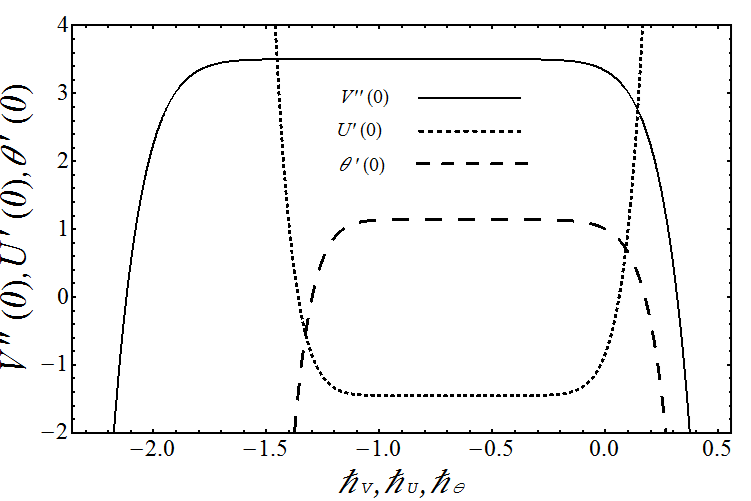
Figure 2. ℏ- curves of V'(0),U'(0) and θ'(0) at 10^th order of approximate for β = 0.2, Pr = 0.5, E = 0.5, M = 1.5, Nr = 0.5, and Re = 1

4. HAM Criteria

The best approximation of the considered problem is based on ℏ_V,ℏ_U "and" ℏ_θ . The curves are up to the order 10^th in Figure 2. Moreover, it is observed that these are in the acceptable ranges of ℏ_V, ℏ_u and ℏ_θ , which are -1.7≤ℏ_V≤-0.2, -1.1≤ℏ_u≤-0.2, and -1≤ℏ_θ≤-0.1.

5. Discussion

Based on the analysis, this section is devoted to discuss the solutions of dimensionless velocity and temperature fields. HAM and other numerical techniques have been utilized to find the solution of the problem under consideration. Graphs are drawn for the comparison of these solutions.

Figure 3 is drawn to show the detailed comparison for two different values of slip parameter β for velocity field U(y) and for the chosen points of the magnetic parameter and slip parameter β, putting Re = 1. The figure describes that magnetic field behaves like a retarding force for velocity. In contrast, Figure 4 shows that by means of both solution techniques the magnetic field reduces the normal velocity. Whereas, the reverse situation is observed for discrete values of the slip parameter  

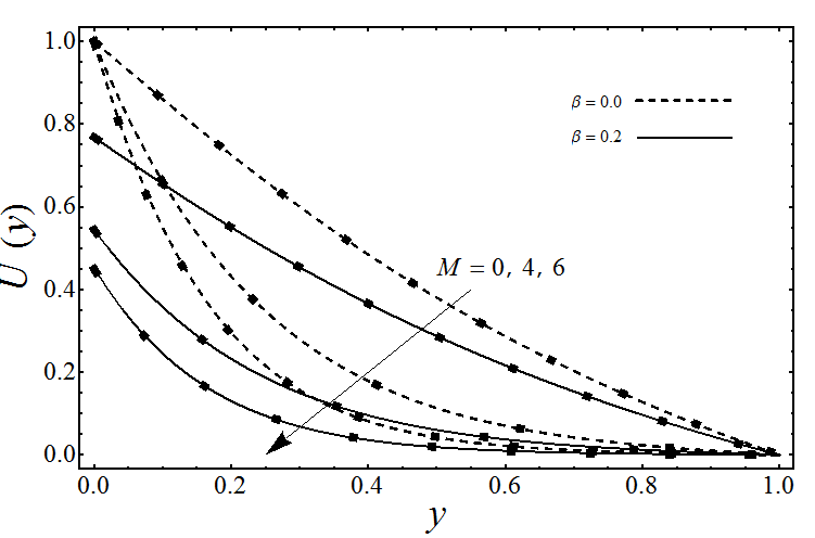
Figure 3. Analysis of numerical solution (filled square) and ham solution (solid and dashed lines) U(y) for and for distinct points of magnetic parameter and slip parameter β when Re = 1.

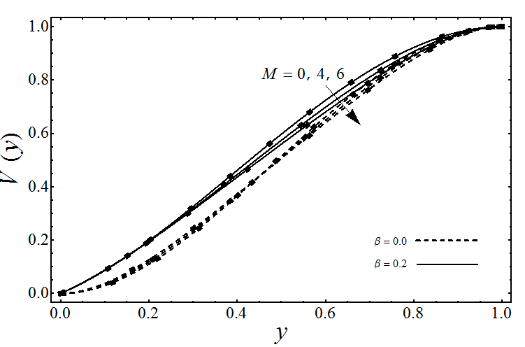
Figure 4. Analysis of numerical solution (filled square) and HAM solution (solid and dashed lines) V(y) for and for discrete points of magnetic parameter M and slip parameter β when Re = 1.

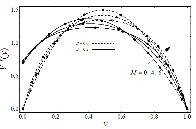
Figure 5. Analysis of numerical solution (filled square) and HAM solution (solid and dashed lines )V'(y) for and for distinct points of magnetic parameter M and slip parameter β when Re = 1.

The accuracy of HAM and numerical solution is depicted in Figure 5 for V'(y) , for different values of the magnetic parameter M, and for the two fixed values of β. It is evident from this figure that for β = 0 and for the modest values of M, the viscosity influences the induction drag and V'(y) is nearly parabolic for M = 0. For higher values of M, the viscosity remains uncritical and its influence is bound to a thin boundary layer near the wall. For β = 0.2 and by increasing the value of M, the maximum velocity point is moved over to the solid wall and its value is increased.

Figures 6-8 show insight into the impacts of different emerging parameters on the temperature field for β = 0 and β = 0.2. The temperature of fluid shows the decreasing behavior for the increasing values of β.

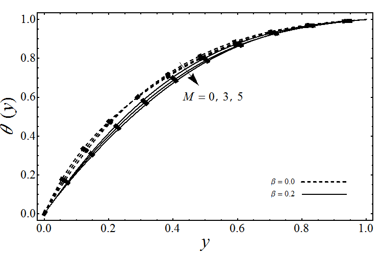
Figure 6. Analysis of numerical solution (filled square) and HAM solution (solid and dashed lines) for  and for various points of slip parameter β and magnetic parameter M when Re = 5, Nr = 0.1, Pr = 1, and E = 1.

Figure 6 demonstrates the comparison of the two solution techniques for the temperature field. A decrease is noticed in the value of temperature for greater values of M. Figure 7 shows the accuracy of and comparison between the two solution methods regarding the various values of temperature and the Prandtl number, when the other factors are kept constant. It can be seen that the increase in the temperature of the fluid causes an increase in the value of the Prandtl number. Figure 8 highlights that the behavior of two solutions regarding the temperature distribution for distinct values of the radiation parameter Nr is aggravated. Notably, the value of the temperature of the fluid reduces as the value of Nr increases. This is due to the fact that $\mathrm{Nr}=\frac{16{\sigma }^{*}{T}_{\infty }^3}{3k{k}^{*}}$ indicates the relative contribution of thermal conduction to thermal radiation. As the value of Nr increases, the effects of thermal conduction become more significant than thermal radiation. So, a decrease in thermal radiation due to an increase in the value of Nr corresponds to depleting the thermal diffusion of the fluid regime and decreasing the thermal energy. Hence, the temperature of the fluid decreases.

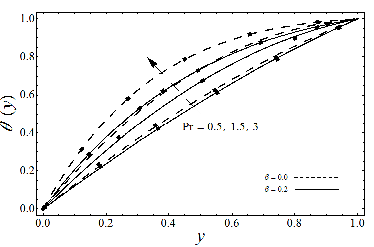
Figure 7. Analysis of numerical solution (filled square) and HAM solution (solid and dashed lines) for θ(y) and for various points of slip parameter β and Prandtl number Pr when Re = 1, M = 1.5, Nr = 0.1, and E = 1.

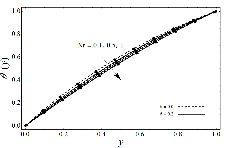
Figure 8. Analysis of numerical solution (filled square) and HAM solution (solid and dashed lines) for θ(y) and for different points of slip parameter β and radiation parameter Nr when Re=1, M = 1.5, Pr = 1, and E = 0.5.

A comparative study of numerical and analytical solutions is presented through graphs. The comparisons of analytical and numerical solutions are found to be in excellent agreement. The study shows that due to an increase in the values of M and β, a decrease is observed in U(y),V(y) and θ(y) whereas an increase is noticed forV'(y) . An increase in temperature is noted for large values of Pr and β but the situation no longer remains the same in the case of Nr.

CONFLICT OF INTEREST

The authors of the study have no financial or non-financial conflict of interest in the subject matter or materials discussed in this study.

DATA AVAILABILITY STATEMENT

Data availability is not applicable as no new data has been created.

FUNDING DETAILS

There are no funding resources dedicated for this research.

REFERENCES

- Huang Y, Zhang H, Yang X, Shen JW, Guo, Y. A review: current urea sorbents for the development of a wearable artificial kidney. J Mater Sci. 2024;59:11669–11686. https://doi.org/10.1007/s10853-024-09898-6
- Wickramasinghe SR, Han B. Designing microporous hollow fibre blood oxygenators. Chem Eng Res Des. 2005;83(3):256–267. https://doi.org/10.1205/cherd.04195
- Jafari A, Mousavi SM, Kalari P. Numerical investigation of blood flow. Part I: In microvessel bifurcations. Commun Nonlin Sci Numer Simul. 2008;13(8):1615–1626. https://doi.org/10.1016/j.cnsns.2006.09.017
- Kamışlı K. Laminar flow of a non-Newtonian fluid in channels with wall suction or injection. Int J Eng Sci. 2006;44(10):650–661. https://doi.org/10.1016/j.ijengsci.2006.04.003
- Saqib M, Khan I, Shafie S. Application of Atangana-Baleanu fractional derivative to MHD channel flow of CMC-based-CNT's nanofluid through a porous medium. Chaos Solit Frac. 2018;116:79–85. https://doi.org/10.1016/j.chaos.2018.09.007
- Saqib M, Khan I. Shafie S. Application of fractional differential equations to heat transfer in hybrid nanofluid: modeling and solution via integral transforms. Adv Differ Equ. 2019;2019:e52. https://doi.org/10.1186/s13662-019-1988-5
- Hussnan A, Khan I, Dalleh Z. Slip effects on unsteady free convective heat and mass transfer flow with newtonian heating. Therm Sci. 2016;20(6):1939–1952. https://doi.org/10.2298/TSCI131119142A
- Saqib M, Khan I, Chu YM, Qushairi A, Shafie S, Nisar KS. Multiple fractional solutions for magnetic bio-nanofluid using oldroyd-b model in a porous medium with ramped wall heating and variable velocity. Appl Sci. 2020;10(11):e3886. https://doi.org/10.3390/app10113886
- Saqib M, Shafie S, Khan I, Chu YM, Nisar KS. Symmetric MHD channel flow of nonlocal fractional model of BTF containing hybrid nanoparticles. Symmetry. 2020;12(4):e663. https://doi.org/10.3390/sym12040663
- Saqib M, Kasim ARM, Mohammad NF, Ching DLC, Shafie S. Application of fractional derivative without singular and local kernel to enhanced heat transfer in CNTs nanofluid over an inclined plate. Symmetry. 2020;12(5):e768. https://doi.org/10.3390/sym12050768
- Saqib M, Hanif H, Abdeljawad T, Khan I, Shafie S, Nisar KS. Heat transfer in MHD flow of Maxwell fluid via fractional cattaneo-friedrich model: a finite difference approach. Comput Mat Cont. 2020;65(3):1959–1973. https://doi.org/10.32604/cmc.2020.011339
- Hussanan A, Salleh MZ, Khan I, Shafie S. Analytical solution for suction and injection flow of a viscoplastic Casson fluid past a stretching surface in the presence of viscous dissipation. Neural Comput Appl. 2018;29:1507–1515. https://doi.org/10.1007/s00521-016-2674-0
- Hussanan A, Khan I, Gorji MR, Khan WA. CNTs-water–based nanofluid over a stretching sheet. 2019;9:21–29. https://doi.org/10.1007/s12668-018-0592-6
- Ziabakhsh Z, Domairry G. Solution of the laminar viscous flow in a semi-porous channel in the presence of a uniform magnetic field by using the homotopy analysis method. Comm Nonlin Sci Num Simul. 2009;14(4):1284–1294. https://doi.org/10.1016/j.cnsns.2007.12.011
- Rundora L, Makinde OD. Effects of Navier slip on unsteady flow of a reactive variable viscosity non-Newtonian fluid through a porous saturated medium with asymmetric convective boundary conditions. J Hydrodym Ser. 2015;27(6):934–944. https://doi.org/10.1016/S1001-6058(15)60556-X
- Sheikholeslami M, Gorji-Bandpy M, Ganji DD. Lattice Boltzmann method for MHD natural convection heat transfer using nanofluid. Powder Technol. 2014;254:82–93. https://doi.org/10.1016/j.powtec.2013.12.054
- Abbas Z, Ahmad B, Ali S. Chemically reactive hydromagnetic flow of a second grade fluid in a semi-porous channel. J Appl Mech Tech Phy. 2015;56(5):878–888. https://doi.org/10.1134/S0021894415050156
- Liao SJ. Beyond Perturbation: Introduction to Homotopy Analysis Method. Chapman and Hall/CRC Press; 2003.
- Liao SJ. On the homotopy analysis method for nonlinear problems. Appl Math Comput. 2004;147(2):499–513. https://doi.org/10.1016/S0096-3003(02)00790-7
- Liao SJ, Campo A. Analytic solution of the temperature distribution in Blasius viscous flow problems. J Fluid Mech. 2002;453:411–425. https://doi.org/10.1017/S0022112001007169