Finite Fractional Hilbert Transform

1. INTRODUCTION

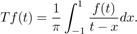
The finite Hilbert transform, when it exists, is defined as [1]

                                                                                (1)

In contrast to Hilbert transform, Cauchy’s principal integral for finite Hilbert transform is over a finite interval. In the literature [2, 3], this finite interval is mostly assumed to be (−1,1). Some of its properties, for example, linearity, boundedness, and Parseval’s formula, follow directly from the Hilbert transform. However, some other properties of the finite Hilbert transform cannot be deduced from the infinite transform. As an example, the inverse of the finite Hilbert transform is not unique and depends on the function f(t). The finite Hilbert transform has been studied extensively based on its applications in the theory of aerodynamics, namely the airfoil equation, image reconstruction, and for its own interest. Its extension and inverse have been investigated in [3–6].

The fractional Hilbert transform was introduced by Lohmann, Mendlovic, and Zalevsky [7]. Cusmariu and Zayed have given alternative definitions of fractional Hilbert transform [8–11]. The fractional Hilbert transform of a function f ∈ (1 ≤ p < ∞) is defined as [11]

for α  0, π/2, π.                (2)

The reader is referred to [12–16] for a detailed discussion on fractional Hilbert transform.

The following results play a vital role in the study of fractional Hilbert transform. These well-known results will be of use in later applications.

Let f ∈ L^p for p > 1, and g ∈ L^q such that (1/p) + (1/q) = 1. Then

                                                (3)

                                                 (4)

For f ∈ L^p for p > 1, the fractional Hilbert transform satisfies

∥H_α f ∥_p ≤ ∥f ∥_p

where

Definition 1 [18] A function f : [−1,1] → R is called β− Hölder continuous on (−1,1) if for all x, t ∈ (−1,1) and 0 < β ≤ 1, there exists any constant H >0 such that

|f(x) − f(t)| ≤ H .

Clearly,  is a continuous function that satisfies Hölder’s inequality.

The following result holds.

Theorem 2 [19] If f is a β− Hölder continuous on (−1,1) then

In the present paper, we define the finite fractional Hilbert transform. Further, we consider some of its identities that play a vital role in the study of this transform. Moreover, some results of the finite Hilbert transform in [1] are modified. Plots for the functions of interest are also provided. The organization of the paper is as follows. In Section 2, we define finite fractional Hilbert transform. In Section 3, we discuss Parseval-type identities. In Section 4, we study the boundedness of finite fractional Hilbert transform. Finally, plots for functions of interest are provided.

2. FINITE FRACTIONAL HILBERT TRANSFORM

In the present paper, we introduce the following definition of finite fractional Hilbert transform Tα of f ∈ Lp (1 ≤ p < ∞) as

which exists a.e. for t ∈ (−1,1).

It is a generalization of the finite Hilbert transform. It satisfies the linearity and boundedness properties which can be deduced from the fractional Hilbert transform and can be easily proved. However, some results are indispensable for the further study of finite fractional Hilbert transform. The local properties of the fractional Hilbert transform can be well understood from the finite fractional Hilbert transform. Therefore, the proposed finite fractional Hilbert transform can have applications in image reconstruction besides pure mathematical interest.

3. Results

The following results hold.

Theorem 3 Let f ∈ L^p and g ∈ L^q such that p > 1, q > 1, and . If both f and g vanish identically outside of the interval (−1,1), then

Proof: The proof of the first equation follows directly from the Parseval-type identity for the fractional Hilbert transform 3.

The second equation is an analog for the modified Parseval-type identity provided for the finite Hilbert transform [7].

Many authors have investigated inequalities for the finite Hilbert transform [20]. In this section, we obtain an inequality for the finite fractional Hilbert transform of a β−Hölder continuous function which is a modification of the result in [19].

Theorem 4 Let f ∈ L^p be a β−Hölder continuous function on (−1,1), such that T_α [f (t)] exists for all t ∈ (−1,1). Then

  (9)

for all x,t ∈ (−1,1).

Proof:

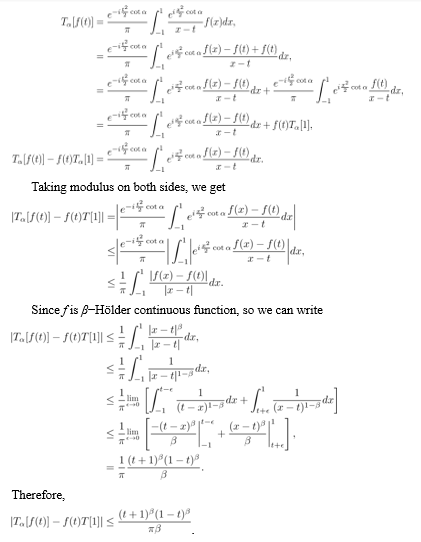
Using Inequality 5 gives us the second inequality. Thus,

This completes the proof. Using triangle inequality for complex numbers, we can state and prove the following basic result which gives us bounds for finite fractional Hilbert transform.

Theorem 5 Let f ∈ L^p such that T_α [f (t)] exists for all t ∈ (−1,1), then we have the inequality

4.  Numerical EXAMPLES

By using Inequality 10 we define the lower bound for finite fractional Hilbert transform as

l[f (t)] = |T_α[f (t)]| − |f (t)T_α[1]|,

the upper bound as

U[f (t)] = |T_α[f (t)]| + |f (t)T_α[1]|,

and |T_α[f (t)] – f (t)T_α[1]| by D[f (t)]. If we consider the function f : [−1,1] → R, f (t) = e^t, then it can be seen in Figure 1 that the plots of l[f (t)],D[f (t)],U[f (t)] are close to each other. Figure 2 contains plots l[f (t)],D[f (t)],U[f (t)] for f (t) =  . For the function f(t) = sin(t), Figure 3 contains plots l[f (t)],D[f (t)],U[f (t)].

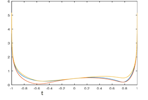
Figure 1. For α=π/4, Plots of a Lower Bound, The Difference D[f (t)] and an Upper Bound for T_α[e^t].

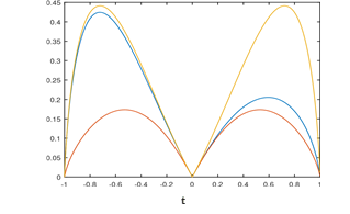
Figure 2. For α=π/4, Plots of a Lower Bound, The Difference D[f (t)] and an Upper Bound for T_α [√(t^2+1)].

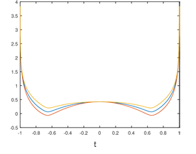
Figure 3. For α=π/4, Plots of a Lower Bound, The Difference D[f (t)] and an Upper Bound for T_α [〖sin(〗⁡t)].

5. CONCLUSION

The current paper’s definition of the finite fractional Hilbert transform and the discussion of boundedness and linear properties are its main contributions. All Hilbert transforms, including the classical Hilbert transform, the finite Hilbert transform, the fractional Hilbert transform, and the finite fractional Hilbert transform, are linear transforms according to their linear property. Another contribution of the paper is that we have proved bounds for the finite fractional Hilbert transform and studied numerical examples.

In future research, an inversion of the finite fractional Hilbert transform can be proven. We propose that the readers study the expansion of the finite fractional Hilbert transform on  and  spaces.

Author Contribution

Naheed Abdullah: Conceptulization, Writing-original draft, writing-review & editing. Saleem Iqbal: Supervision. Abdul Rehman: Methodology

Conflict of Interest

The authors of the manuscript have no financial or non-financial conflict of interest in the subject matter or materials discussed in this manuscript.

REFERENCES

- King FW, Hilbert Transforms. Cambridge: Cambridge University Press; 2009. https://doi.org/10.1017/CBO9780511721458
- Curbera GP, Okada S, Ricker WJ. Fine spectra of the finite Hilbert transform in function spaces. Adv Math. 2021;380:e107597. https://doi.org/10.1016/j.aim.2021.107597
- Giang DV. Finite Hilbert transforms. J Approx Theory. 2015;200:221-226. https://doi.org/10.1016/j.jat.2015.08.001
- Curbera GP, Okada S, Ricker WJ. Inversion and extension of the finite Hilbert transform on (−1,1). Ann Mat Pura Appl. 2019;198:1835-1860. https://doi.org/10.1007/s10231-019-00837-w
- Curbera GP, Okada S, Ricker WJ. Extension and integral representation of the finite Hilbert transform in rearrangement invariant spaces. Quaest Math. 2020;43(5-6):783-812. https://doi.org/10.2989/16073606.2019.1605423
- Curbera GP, Okada S, Ricker WJ. Non-extendability of the finite Hilbert transform. Monatsh Fur Math. 2021;195:649–657. https://doi.org/10.1007/s00605-021-01572-2
- Lohmann AW, Mendlovic D, Zalevsky Z. Fractional hilbert transform. Opt Lett. 1996;21(4):281-283. https://doi.org/10.1364/OL.21.000281
- Cusmariu A. Fractional analytic signals. Signal Process. 2002;82(2):267-272. https://doi.org/10.1016/S0165-1684(01)00186-4
- Davis JA, McNamara DE, Cottrell DM. Analysis of the fractional Hilbert transform. Appl Opt. 1998;37(29):6911-6913. https://doi.org/10.1364/AO.37.006911
- King FW. Hilbert Transforms. Cambridge: Cambridge University Press; 2009. https://doi.org/10.1017/CBO9780511735271
- Zayed AI. Hilbert transform associated with the fractional Fourier transform. IEEE Signal Process Lett. 1998;5(8):206-208. https://doi.org/10.1109/97.704973
- Abdullah N, Iqbal S. The fractional Hilbert transform of generalized functions. Symmetry. 2022;14(10):e2096. https://doi.org/10.3390/sym14102096
- Guanlei X, Xiaogang X, Xiaotong W. Generalized entropic uncertainty principles on the complex signals in terms of fractional Hilbert transform. Optik, 2020;216:e164966. https://doi.org/10.1016/j.ijleo.2020.164966
- Poularikas AD. Transforms and Applications Handbook. CRC Press; 2018. https://doi.org/10.1201/9781315218915
- Venkitaraman A, Seelamantula CS. Fractional Hilbert transform extensions and associated analytic signal construction. Signal Process. 2014;94:359-372. https://doi.org/10.1016/j.sigpro.2013.05.009
- Zayed AI. Handbook of Function and Generalized Function Transformations. CRC Press; 2019. https://doi.org/10.1201/9780138752859
- Abdullah N, Iqbal S, Khalid A, et al. The fractional Hilbert transform on the real line. Math Prob Eng. 2022;2022:1-11. https://doi.org/10.1155/2022/5027907
- Dragomir SS. Inequalities and approximations for the Finite Hilbert transform: a survey of recent results. In: Rassias TM, Pardalos PM, eds. Mathematical Analysis and Applications. 2019;53-164. https://doi.org/10.1007/978-3-030-31339-54
- Dragomir SS. Some inequalities for the finite Hilbert transform of a product. Korean Math Soc. 2003;18(1):39-57. https://doi.org/10.4134/CKMS.2003.18.1.039
- Dragomir SS. Inequalities for the finite Hilbert transform of convex functions. J Numer Anal Approx Theory. 2019;48(2):148-158. https://doi.org/10.33993/jnaat482-1177