

| Review | Open Access |
|---|
Convergence and Ulam-Hyers-Rassias Stability Analyses of Numerical Solutions of Bratu Type Equations using Picard Method |
 |
|---|
 Saif Ullah*,
Muzaher Ali,
Sana Bajwa, and
Ahsan Bilal
Saif Ullah*,
Muzaher Ali,
Sana Bajwa, and
Ahsan Bilal
1Institute of Industrial Biotechnology, Government College University, Lahore, Pakistan
2Institute of Microbiology and Molecular Genetics, University of the Punjab, Lahore, Pakistan
The Bratu equation is a basic nonlinear boundary value problem with important applications to fuel ignition, thermal combustion, and nanotechnology. The current article presents a new application of the Picard iterative technique to find accurate approximate solutions for this equation. Firstly, the conditions for existence and uniqueness of the solutions are determined. Furthermore, the article provides an explicit formulation of Picard’s scheme for second-order ordinary differential equations and its particular implementation to the Bratu type problem. The iterative solutions obtained are analyzed thoroughly for convergence and are proved to be Ulam-Hyers-Rassias stable, a very strong type of stability not yet known for these kind of solutions. Numerical tests for three cases ( 𝜇 = 1 , 2, and the critical value 𝜇 = 3.51383 ) are shown to exemplify outstanding accuracy of the proposed approach. A thorough comparison with known techniques including the Adomian Decomposition Method, Homotopy Perturbation Method, and Variational Iteration Method indicates that the Picard iterative scheme is much better in terms of accuracy since its maximum absolute errors are much smaller.
Highlights
- The foremost aim of the current article is to compute approximate solutions of BTEs using Picard’s method which are new and not described before in the literature.
- The convergence of the sequence 𝑈𝑛(𝑥), generated by Picard’s iteration is assessed using the uniform convergence criterion on the interval 𝑥 ∈ [0, 1].
- This demonstrates that both exact and Picard’s solutions make an excellent agreement.
1. INTRODUCTION
Mathematical modeling of many physical phenomena is achieved in the form of integral equations, differential equations (DEs), or integro- differential equations [1-3]. Bratu type DEs have many applications in practical life. These include fuel ignition, Chandrasekhar model, nanotechnology, thermal reaction, heat transfer by conduction, radiative heat transfer, and chemical reactor theory [4-7]. The scientists and researchers are very keen in the study of Bratu type equations (BTEs). This is because the solutions of such type of equations are more natural and significant due to their important usage in engineering and scientific experimentations. The following equation is called one dimensional Bratu equation [8, 9]
𝑈′′(𝑥) + 𝜇 𝑒𝑈(𝑥) = 0 with 𝑈(0) = 0, 𝑈(1) = 0 ; ∀ 𝑥 ∈
[ 0, 1] (1)
where 𝜇 > 0 is a physical parameter. Exact solution of above equation (1) is10]

Several analytical, semi-analytical, and numerical schemes have been used to solve BTEs. Decomposition Method (DM) [11], Homotopy Perturbation Method (HPM) [12, 13], Perturbation Iteration Algorithm (PIA) [14], Optimal Homotopy Asymptotic Method (OHAM) [15], Laplace Method (LM) [16], Variational Iteration Method (VIM) [17], Perturbation Method (PM) [18], and B Spline Method (BSM) [19] have been implemented to handle BTEs.
While the above-mentioned approaches have been used successfully, they require intricate calculations, for instance, the formation of Adomian
polynomials or determining auxiliary parameters and functions in homotopy-based approaches. The Picard iterative scheme is an attractive alternative considering its simplicity of concept, ease of implementation, and well-established rapid convergence for many nonlinear problems [20-24]. However, its use on the Bratu equation, especially with an extensive study on the stability of its solutions, is an uncharted territory. Therefore, the current article aimed to fill that gap. The novelty of this research is two-pronged: (i) systematic use and numerical verification of the Picard method for BTEs and (ii) pioneering Ulam-Hyers-Rassias stability study of the approximate solutions developed by the iterative scheme.
The study of Ulam-Hyers type stability of various dynamical systems has received considerable attention. The famous Ulam-Hyers stability instigated in a seminar at the Wisconsin University in 1940, where Ulam
[25] suggested the problem of the stability for functional equations. A significant development occurred in 1941, when Hyers [26] gave a partial solution to Ulam’s problem. After an in-depth analysis of the Ulam-Hyers stability structure, some researchers extended and used the concept of Ulam-Hyers stability, such as generalized Ulam-Hyers stability [27, 28], Ulam-Hyers-Rassias stability [29], and generalized Ulam-Hyers-Rassias stability. Huang et al. [30] analyzed Hyers-Ulam stability, while Qarawani
[31] investigated Hyers-Ulam-Rassias stability of nonlinear DEs. Wang et al. considered Ulam-Hyers stability of fuzzy fractional DEs with delay [32, 33].
The foremost aim of the current article is to compute approximate solutions of BTEs using Picard’s method which are new and not described before in the literature. The article is organized as: Section 2 covers conditions for existence and uniqueness of solutions, while section 3 comprehends the illustration of Picard method. Section 4 presents the solutions of numerical examples. The convergence and stability analyses of the derived solutions have been performed in section 5 and 6, respectively. Estimation of error and comparison of results are incorporated in section 7, while conclusion of the article is drafted in section 8.
2. CONDITIONS FOR EXISTENCE AND UNIQUENESS OF SOLUTIONS OF BRATU EQUATIONS
The existence and uniqueness of solutions for the Bratu problem are well-established and depend critically on the parameter 𝜇 . The
foundational result is summarized in the following theorem:
Theorem 1. There are three cases for μ given in equation (1)
- If 𝜇 = 𝜇0, then there exists one solution,
- If 𝜇 < 𝜇0, then there exist two solutions,
- If 𝜇 > 𝜇0, then no solution
Here 𝜇0 is called the critical value [12, 13] given as:
1 =1/4� 2 𝜇0 sinh (4),
and its numerical value is
𝜇0 = 3.513830719.
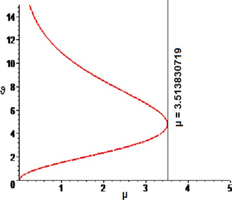
Figure 1. Comparison of 𝜇 and 𝖯.
Figure 1 shows that when 𝜇 < 3.513830719, then 𝖯 has two values for each value of 𝜇. Hence, there are two solutions for each
𝜇 < 3.513830719. For 𝜇 = 3.513830719, only one value of
𝖯 = 4.798645359 exists and there is a unique solution. When
𝜇 > 3.513830719, there is no resultant value of 𝖯, and in this case, no solution of Bratu equation exists [12, 13].
3. DESCRIPTION OF PICARD METHOD
This section discusses the description of Picard method for second- order ordinary differential equation (ODE) and its implementation to BTE.
3.1. Formulation of Picard Method for Second-Order ODE
that is Picard’s iterative scheme for second-order ODE [21, 22].
3.2. Implementation to Bratu Equation
From the above equation (6), we have [12, 34]


which is the exact solution of equation (10). Taking 𝑈0(𝑥) = 0 and applying Picard method, we get
𝑈1(𝑥) = 0.5493527280 𝑥 − 0.5 𝑥2 ,
𝑈2(𝑥) = 0.0003720238095 𝑥8 − 0.001634978357 𝑥7 − 0.001651763169 𝑥6
+0.01235224910 𝑥5 + 0.02909214918 𝑥4 − 0.09155878800 𝑥3 − 0.5 𝑥2
+0.5493527280 𝑥,
and
U3 (x) = 0.5493527280 x − 0.5 x2 − 0.09155878800 x3 + 0.02909214918 x4 + 0.0183117576 x5 − 0.003459802640 x6 −
0.001764607014 x7 + 0.9322482480 × 10−4x8 +
1.580853532 × 10−4x9 + 0.4533942348 × 10−5x10 −
1.393134891 × 10−5x11 + 0.06120893625 × 10−6x12 +
0.06540389326 × 10−5x13 + + 0.04400289 × 10−6x14 −
0.03474251 × 10−6x15 − 0.03008674 × 10−7x16 +
0.02236216459 × 10−7 x17 − 0.02261465929 × 10−8 x18
(13)
that is the approximate solution of equation (10).
4.2. Example-2
which is the exact solution of equation (14). Taking 𝑈0(𝑥) = 0 and applying Picard method, we get
𝑈1(𝑥) = 1.248217518 𝑥 − 𝑥2 ,
𝑈2(𝑥) = 0.005952380952 𝑥8 − 0.02971946472 𝑥7
+0.01860156574 𝑥6 + 0.0924087264 𝑥5 + 0.0368294189 𝑥4
−0.416072506 𝑥3 − 𝑥2 + 1.248217518 𝑥, (16)
and
𝑈3(𝑥) = −0.115787055 × 10⁻⁶ 𝑥18 + 0.130074688 × 10⁻⁵ 𝑥17 − 0.460289 × 10⁻⁵ 𝑥16
−0.02644413 × 10⁻⁶ 𝑥15 + 0.2586929702 × 10⁻⁴ 𝑥14 + 0.2374648306 × 10⁻⁴ 𝑥13
−0.1722400368 × 10⁻³ 𝑥12 − 0.5966016460 × 10⁻³ 𝑥11 + 0.001944801524 𝑥10
+0.003173141654𝑥9 − 0.00655987510 𝑥8 − 0.02640249326 𝑥7 − 0.001165361882 𝑥6
+0.1664290024 𝑥5 + 0.03682941898 𝑥4 − 0.4160725060 𝑥3 − 𝑥2 + 1.248217518 𝑥 ,
(17)
that is the approximate solution of equation (14).
4.3. Example-3
Thus,
cosh ([𝑥 − 0.5] 4.798645359)
𝑈(𝑥) = −2ln (cosh ([𝑥 − 0.5] 4.798645359/ 2 )) ,
cosh (4.798645359/4)
⇒ 𝑈(𝑥) = −2 ln(0.5524420911cosh(2.399322680 𝑥 − 1.199661340)),
which is the exact solution of equation (18). Taking 𝑈0(𝑥) = 0 and applying Picard method, we get
𝑈1(𝑥) = 3.999916982 𝑥 − 0.5 𝑥2 ,
𝑈2(𝑥) = 0.00130722869 𝑥8 − 0.04183044990 𝑥7 + 0.4538503540 𝑥6 − 1.5225505 𝑥5
−2.196046963 𝑥4 − 2.342505194 𝑥3 − 1.756915360 𝑥2 + 3.999916982 𝑥 ,
𝑈3(𝑥) = −2.405744959 × 10⁻³𝑥18 + 6.295431774 × 10⁻³𝑥17 + 6.06359428 × 10⁻³𝑥16
−0.04140070848 𝑥15 + 0.2133926181 𝑥14 − 0.3033346185 𝑥13 − 0.1635341992 𝑥12
−0.2943933311 𝑥11 − 1.238108848 𝑥10 − 0.09860541020 𝑥9 + 0.06549570825 𝑥8
+1.569248472 𝑥7 + 2.820111160𝑥6 − 0.2276930256 𝑥5 − 1.827997980 𝑥4
−2.342505194 𝑥3 − 1.756915360 𝑥2 + 3.999916982 𝑥, (20)
and
𝑈4(𝑥) = 3.999916982 𝑥 − 1.756915360 𝑥2 − 2.342505194 𝑥3 −
2.608816838 𝑥4 + 2.057791678 𝑥5 + 1.436367948 𝑥6 +
0.3755924260 𝑥7 − 0.5989937866 𝑥8 − 1.115268983 𝑥9 −
0.1861262692 𝑥10 + 0.4014073533𝑥11 + 0.4895580669𝑥12
−0.2133778426𝑥13 − 0.1783860287𝑥14 − 0.2345269362𝑥15 −
0.110694331 𝑥16 + 0.0325434749 𝑥17 + 0.0946829798 𝑥18 +
0.0545570354 𝑥19 + 0.023638545𝑥20 − 0.0242938671 𝑥21 −
0.021804040 𝑥22 + 0.0072424414 𝑥23 + 0.0741606236 𝑥24 +
0.002463820 𝑥25 − 0.0059534466 𝑥26 − 0.0012045626 𝑥27 −
0.0067346123 𝑥28 − 0.0011077633 𝑥29 + 0.00771358043𝑥30 +
0.000802098𝑥31 + 0.0003443211𝑥32 + 0.61416749 × 10⁻⁵ 𝑥33 −
0.0201121798 × 10⁻⁵ 𝑥34 − 0.0922424728 × 10⁻⁵ 𝑥35 −
0.16190965120 × 10⁻⁶ 𝑥36 + 0.056308070 × 10⁻⁶ 𝑥37 + 0.00429760 ×
10−7 𝑥38 + 0.0748094200 × 10⁻⁷ 𝑥39 − 0.0306817000 × 10⁻⁷𝑥40 −
0.03965400 × 10⁻⁸ 𝑥41 + 0.05616 × 10⁻⁹ 𝑥42 − 0.01964754709 ×
10−9 𝑥43 + 0.041984642179 × 10⁻⁹ 𝑥44 − 0.064080398 × 10⁻¹⁰ 𝑥45 +
0.07435209 × 10⁻¹¹ 𝑥46 − 0.067626903 × 10⁻¹² 𝑥47 + 0.0489542041 ×
10−13 𝑥48 − 0.0283546 × 10⁻¹⁴ 𝑥49 + 0.013108496 × 10⁻¹⁵ 𝑥50 −
0.0047865113 × 10⁻¹⁶ 𝑥51 + 0.013534696 × 10⁻¹⁷ 𝑥52 − 0.0286394 ×
10−19 𝑥53 + 0.04273016 × 10⁻²³ 𝑥54 − 0.40268047 × 10⁻²⁵ 𝑥55 +
0.17958767 × 10⁻²⁷ 𝑥56. (21)
that is the approximate solution of equation (18).
4.4. Example-4Consider
𝑈′′(𝑥) + 5 𝑒𝑈(𝑥) = 0 with 𝑈(0) = 0 , 𝑈(1) =
0 ; ∀ 𝑥 ∈ [ 0 , 1]. (22)
Here, 𝜇 = 5. To find the solutions of above equation (22)
𝑈(𝑥) = −2ln (cosh(|𝑥-0.5|P/2)/cosh(p/4)
and 𝖯 can be derived from
𝖯 = √2 × 5 cosh (P/4).
Since 𝜇 = 5, then
𝖯 = √2 × 5 cosh (P/4) (23)
After solving equation (23), we get
𝖯 = (−3.181805553 + 5.282305940 𝑖 )√10.
Since 𝖯 is a complex number, therefore it can not be continued further. It has already been deliberated upon that for 𝜇 > 3.513830719, Bratu equation has no solution.
5. CONVERGENCE ANALYSIS
This section discusses the convergence of solutions of numerical examples derived by Picard method.
5.1. Convergence CriteriaThe convergence of the sequence 𝑈𝑛(𝑥) generated by Picard’s iteration
is assessed using the uniform convergence criterion on the interval 𝑥 ∈ [𝟎𝟎, 1]. Recall that a sequence of functions 𝑈𝑛(𝑥) converges uniformly to a function 𝑈(𝑥) if [35]
lim 𝑠𝑢𝑝|𝑈𝑛(𝑥) − 𝑈(𝑥)| = 0.
𝑛→∞
It will be demonstrated numerically that for given examples, the maximum absolute error |𝑈𝑛(𝑥) − 𝑈(𝑥)| indeed decreases below a predefined tolerance 𝜀𝜀 after a finite number of iterations 𝑛, providing strong empirical evidence for uniform convergence.
5.2. Convergence Analysis of Solution of Example-1Since it has been discussed above that 𝑈𝑛(𝑥) is uniformly convergent if and only if
sup| 𝑈𝑛(𝑥) − 𝑈(𝑥)| = ∥ 𝑈𝑛(𝑥) − 𝑈(𝑥) ∥ < 𝜀𝜀
when 𝑚 < 𝑛 , ∀ 𝑥 ∈ [ 0 , 1] .
Taking 𝜀𝜀 = 0.00009, we have
sup| 𝑈𝑛(𝑥) − 𝑈(𝑥)| = ∥ 𝑈𝑛(𝑥) − 𝑈(𝑥) ∥ = Max Error < 𝜀𝜀
when 𝑚 < 𝑛 , ∀ 𝑥 ∈ [ 0 , 1]
which implies that 𝑈𝑛(𝑥) converges to 𝑈𝑛(𝑥) , where 𝑚 = 2 and 𝑈(𝑥)
represents exact solution.
5.3. Convergence Analysis of Solution of Example-2Since it has been discussed above that 𝑈𝑛(𝑥) is uniformly convergent if and only if
sup| 𝑈𝑛(𝑥) − 𝑈(𝑥)| = ∥ 𝑈𝑛(𝑥) − 𝑈(𝑥) ∥ < 𝜀𝜀
when 𝑚 < 𝑛 , ∀ 𝑥 ∈ [ 0 , 1] .
Taking 𝜀𝜀 = 0.0009, we have
sup| 𝑈𝑛(𝑥) − 𝑈(𝑥)| = ∥ 𝑈𝑛(𝑥) − 𝑈(𝑥) ∥ = Max Error < 𝜀𝜀
when 𝑚 < 𝑛 , ∀ 𝑥 ∈ [ 0 , 1]
which implies that 𝑈𝑛(𝑥) converges to 𝑈(𝑥) , where 𝑚 = 2 and 𝑈(𝑥)
represents exact solution.
5.4. Convergence Analysis of Solution of Example-3Since it has been discussed above that 𝑈𝑛(𝑥) is uniformly convergent if
and only if
sup| 𝑈𝑛(𝑥) − 𝑈(𝑥)| = ∥ 𝑈𝑛(𝑥) − 𝑈(𝑥) ∥ < 𝜀𝜀
when 𝑚 < 𝑛 , ∀ 𝑥 ∈ [ 0 , 1] .
Taking 𝜀𝜀 = 0.022414, we have
sup| 𝑈𝑛(𝑥) − 𝑈(𝑥)| = ∥ 𝑈𝑛(𝑥) − 𝑈(𝑥) ∥ = Max Error < 𝜀𝜀
when 𝑚 < 𝑛 , ∀ 𝑥 ∈ [ 0 , 1]
which implies that 𝑈𝑛(𝑥) converges to 𝑈(𝑥), where 𝑚 = 3 and 𝑈(𝑥) is the exact solution.
6. STABILITY ANALYSIS
This section discusses the stability analysis of numerical scheme for BTEs using the following stability criteria.
5.1. Ulam-Hyers-Rassias Stability (Generalized Ulam-Hyres Stability)The general second-order differential equation is considered as
𝜉′′(𝑥) − 𝐺(𝑥 , 𝜉(𝑥) , 𝜉 ′(𝑥)) = 0 with 𝜉(0) =
0 and 𝜉 ′(0) = 0. (24)
Following [29-31], it can be said that equation (24) is Ulam-Hyers-Rassias (UHR) stable with respect to a continuous functions 𝜉(𝑥) if
- | 𝜉′′(𝑥) − 𝐺(𝑥 , 𝜉(𝑥) , 𝜉 ′(𝑥))| ≤ 𝐻(𝑥) ,
- | 𝜉(𝑥) − 𝜁(𝑥)| ≤ 𝑀(𝑥) ,
where 𝜉(𝑥) , 𝜁(𝑥) ∈ 𝐶 2[𝑎, 𝑏] and 𝐻(𝑥), 𝑀(𝑥) are positive continuous functions. Furthermore, 𝐻(𝑥) does not depend on 𝜉(𝑥) and
𝐺(𝑥 , 𝜉(𝑥) , 𝜉 ′(𝑥)).
6.2. Ulam-Hyers-Rassias Stability of Bratu EquationTheorem 2. The Bratu equation is Ulam-Hyers-Rassias stable, if it fulfills the conditions given below
- � 𝑈𝑛′′(𝑥) + 𝜇𝑒𝑈𝑛(𝑥)� ≤ 𝐻(𝑥) ,
- | 𝑈𝑛(𝑥) − 𝑈(𝑥)| ≤ 𝑀(𝑥).
While a full theoretical proof is beyond the scope of this numerical study, strong numerical evidence will be provided for the stability of derived approximate solutions. For Picard iterations 𝑈𝑛(𝑥) , it will be numerically verified that these inequalities hold for given examples.
6.3. Stability Analysis of Example-1Consider
𝑈′′(𝑥) + 𝑒𝑈(𝑥) = 0 with 𝑈(0) = 0 , 𝑈(1)
= 0 ; ∀ 𝑥 ∈ [ 0 , 1].
Here, 𝜉(𝑥) = 𝑈3(𝑥) and 𝜁(𝑥) = 𝑈(𝑥), then
� 𝑈3′′(𝑥) + 𝑒𝑈3(𝑥)� ≤ max� 𝑈3′′(𝑥) + 𝑒𝑈3(𝑥)� ≤ 𝐻(𝑥)
and
= 𝑥2 + 0.0038857183 ,
| 𝑈3(𝑥) − 𝑈(𝑥) | ≤ max| 𝑈3(𝑥) − 𝑈(𝑥) | ≤ 𝑀(𝑥)
= 𝑥2 + 0.000089546 .
Hence, Example-1 fulfills the hypothesis of Theorem 2 and is Ulam-Hyers-Rassias stable.
6.4. Stability Analysis of Example-2Consider
𝑈′′(𝑥) + 2 𝑒𝑈(𝑥) = 0 with 𝑈(0) = 0 , 𝑈(1)
= 0 ; ∀ 𝑥 ∈ [ 0 , 1].
Here, 𝜉(𝑥) = 𝑈3(𝑥) and 𝜁(𝑥) = 𝑈(𝑥), then
� 𝑈3′′(𝑥) + 2 𝑒𝑈3(𝑥)� ≤ max� 𝑈3′′(𝑥) + 2 𝑒𝑈3(𝑥)� ≤ 𝐻(𝑥)
and
= 𝑥4 + 0.09701083186 ,
| 𝑈3(𝑥) − 𝑈(𝑥) | ≤ max| 𝑈3(𝑥) − 𝑈(𝑥) | ≤ 𝑀(𝑥)
= 𝑥4 + 0.00082169 .
Thus, Example-2 follows the hypothesis of Theorem 2 and is Ulam-Hyers-Rassias stable.
6.5. Stability Analysis of Example-3Consider
𝑈′′(𝑥) + 3.513830719 𝑒𝑈(𝑥) = 0 with 𝑈(0) = 0 , 𝑈(1)
= 0 ; ∀ 𝑥 ∈ [ 0 , 1].
Here, 𝜉(𝑥) = 𝑈4(𝑥) and 𝜁(𝑥) = 𝑈(𝑥), then
� 𝑈4′′(𝑥) + 3.513830719 𝑒𝑈4(𝑥)� ≤ max� 𝑈4′′(𝑥) + 3.513830719 𝑒𝑈4(𝑥)�
≤ 𝐻(𝑥) = 𝑥6 + 65.60872438 ,
and
|𝑈4(𝑥) − 𝑈(𝑥) | ≤ max| 𝑈4(𝑥) − 𝑈(𝑥) | ≤ 𝑀(𝑥)
= 𝑥6 + 0.022414 .
Thus, Example-3 fulfils the hypothesis of Theorem 2 and is Ulam- Hyers-Rassias stable.
7. RESULTS AND DISCUSSION
Here, the efficacy and veracity of Picard’s iterative scheme has been demonstrated through error’s estimation, comparison of maximum errors, and graphical illustrations of the obtained approximate solutions of BTEs.
7.1. Results of Example-1Table 1 contains |E𝐄𝐄𝐄𝐄𝐄𝐄𝐄𝐄| estimated using Picard method, which shows that 𝐦𝐦𝐦𝐦𝐦𝐦 |E𝐄𝐄𝐄𝐄𝐄𝐄𝐄𝐄| = ∥ E𝐄𝐄𝐄𝐄𝐄𝐄𝐄𝐄 ∥ = 𝟎𝟎. 𝟎𝟎𝟎𝟎𝟎𝟎𝟎𝟎𝟎𝟎𝟎𝟎𝟎𝟎𝟎𝟎𝟎𝟎. The ∥ E𝐄𝐄𝐄𝐄𝐄𝐄𝐄𝐄 ∥ estimated by Picard method, PIA [21], DM [18], HPM [13], and OHAM >[15] are listed in Table 2. It explained that Picard’s method has smallest ∥ E𝐄𝐄𝐄𝐄𝐄𝐄𝐄𝐄 ∥.
Figure 2(a , b) demonstrates the comparison of exact solution with approximate solutions obtained by Picard’s iterative scheme. Figure 2(a) shows that both approximate and exact solutions coincide with each other. Figure 2(b) indicates that approximate solutions of zero to third orders are converging to exact solution. Figure 2(c) illustrates the comparison of solutions obtained by Picard’s iterative scheme, HPM, OHAM, DM, and PIA with the exact solution. This demonstrates that both exact and Picard’s solutions make an excellent agreement, while other solutions diverge from exact solution. Figure 2(d) indicates that Picard’s iterative scheme has least ∥ Error ∥ as compared to other stated techniques.
Table 1. Error Estimation of Example-1
|
x |
Exact Sol. |
Picard’s Sol. |
| Error | |
|---|---|---|---|
|
0.00 |
0.0000000000 |
0.0000000000 |
0.0000000000 |
|
x |
Exact Sol. |
Picard’s Sol. |
| Error | |
|
0.10 |
0.0498467900 |
0.0498468027 |
1.27000 × 10⁻⁸ |
|
0.20 |
0.0891899350 |
0.0891902388 |
3.03800 × 10⁻⁷ |
|
0.30 |
0.1176090956 |
0.1176109762 |
1.88060 × 10⁻⁶ |
|
0.40 |
0.1347902526 |
0.1347966401 |
6.38750 × 10⁻⁶ |
|
0.50 |
0.1405392142 |
0.1405548425 |
1.56280 × 10⁻⁵ |
|
0.60 |
0.1347902526 |
0.1348215219 |
3.12690 × 10⁻⁵ |
|
0.70 |
0.1176090956 |
0.1176641754 |
5.50798 × 10⁻⁵ |
|
0.80 |
0.0891899350 |
0.0892797819 |
8.95460 × 10⁻⁵ |
|
0.90 |
0.0498467900 |
0.0498874514 |
4.06614 × 10⁻⁵ |
|
1.00 |
0.0000000000 |
0.0000000000 |
0.0000000000 |
Table 2. Comparison of Error of Example-1
|
Methods |
Error |
|---|---|
|
Picard’s Method |
0.0000895460 |
|
Perturbation Iteration Algorithm |
0.0011992210 |
|
Decomposition Method |
0.0030154732 |
|
Homotopy Perturbation Method |
0.1431299094 |
|
OHAM |
0.9944206698 |
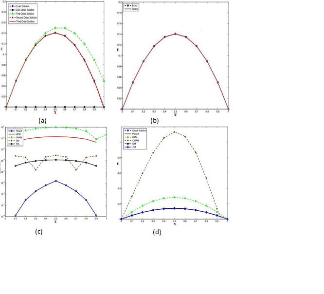
Figure 2. Graphical Illustration of Example-1
7.2. Results of Example-2Table 3 lists | E𝐄𝐄𝐄𝐄𝐄𝐄𝐄𝐄 | estimated by Picard’s iterative scheme. It can be observed that ∥ E𝐄𝐄𝐄𝐄𝐄𝐄𝐄𝐄 ∥ = 𝐦𝐦𝐦𝐦𝐦𝐦 | E𝐄𝐄𝐄𝐄𝐄𝐄𝐄𝐄 | = 𝟎𝟎. 𝟎𝟎𝟎𝟎𝟎𝟎𝟎𝟎𝟎𝟎1𝟎𝟎𝟎𝟎. The ∥ E𝐄𝐄𝐄𝐄𝐄𝐄𝐄𝐄 ∥ estimated by Picard method, Laplace method (LM) [16], DM [18], PIA [14], and HPM [13] drafted in Table 4 indicates that Picard’s method has smallest ∥ E𝐄𝐄𝐄𝐄𝐄𝐄𝐄𝐄 ∥ amongst these methods.
Figure 3(a , b) illustrated the comparison of exact solution with approximate solutions obtained by Picard’s iterative scheme. Figure 3(a) shows that both approximate and exact solutions match with each other. Figure 3(b) shows that approximate solutions of zero to third orders are converging to exact solution. Figure 3(c) demonstrates the comparison of solutions obtained by Picard’s iterative scheme, DM, LM, PIA, and HPM with the exact solution. This illustrates that both exact and Picard’s solutions make an excellent agreement, while solutions derived by other mentioned techniques diverge from exact solution. Figure 3(d) represents that Picard’s iterative scheme has least ∥ Error ∥ as compared to other stated methods.
Table 3. Error Estimation of Example-2
|
x |
Exact Sol. |
Picard’s Sol. |
| Error | |
|---|---|---|---|
|
0.00 |
0.0000000000 |
0.0000000000 |
0.000000000 |
|
0.10 |
0.1144107440 |
0.1144110226 |
7.7860 × 10⁻⁷ |
|
0.20 |
0.2064191156 |
0.2064266804 |
7.5640 × 10⁻⁶ |
|
0.30 |
0.2738793116 |
0.2739270572 |
4.7745 × 10⁻⁵ |
|
0.40 |
0.3150893646 |
0.3152541108 |
1.6474 × 10⁻⁴ |
|
0.50 |
0.3289524214 |
0.3293601056 |
8.2169 × 10⁻⁴ |
|
0.60 |
0.3150893646 |
0.3152541108 |
1.6474 × 10⁻⁴ |
|
0.70 |
0.2738793116 |
0.2739270572 |
4.7745 × 10⁻⁵ |
|
0.80 |
0.2064191156 |
0.2064266804 |
7.5640 × 10⁻⁶ |
|
0.90 |
0.1144107440 |
0.1144110226 |
7.7860 × 10⁻⁷ |
|
1.00 |
0.0000000000 |
0.0000000000 |
0.000000000 |
Table 4. Comparison of Error of Example-2
|
Method |
Error |
|---|---|
|
Picard’s Method |
0.0008216900 |
|
Laplace Method |
0.0123778084 |
|
Decomposition Method |
0.0146751156 |
|
Perturbation Iteration Algorithm |
0.0523780000 |
|
Homotopy Perturbation Method |
0.2559341111 |
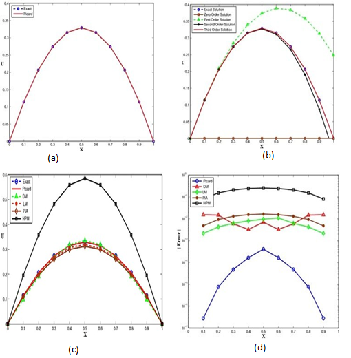
Figure 3. Graphical Illustration of Example-2
7.3. Results of Example-3The | E𝐄𝐄𝐄𝐄𝐄𝐄𝐄𝐄 | estimated by Picard’s iterative scheme is drafted in Table 5 which shows that ∥ E𝐄𝐄𝐄𝐄𝐄𝐄𝐄𝐄 ∥ = 𝐦𝐦𝐦𝐦𝐦𝐦 | E𝐄𝐄𝐄𝐄𝐄𝐄𝐄𝐄 | =𝟎𝟎. 𝟎𝟎𝟎𝟎𝟎𝟎𝟎𝟎1𝟎𝟎. The ∥ E𝐄𝐄𝐄𝐄𝐄𝐄𝐄𝐄 ∥estimated by Picard method, B Spline method [19], HPM [13], PIA [14], and VIM [17] are drafted in Table 6 which shows that Picard method has smallest ∥ E𝐄𝐄𝐄𝐄𝐄𝐄𝐄𝐄 ∥ amongst these methods.
Figure 4 (a, b) represents the comparison of exact solution with approximate solutions obtained by Picard’s iterative scheme. Figure 4(a) shows that both approximate and exact solutions match with each other. Figure 4(b) shows that approximate solutions of zero to fourth orders are converging to exact solution. Figure 4(c) illustrates a comparison of approximate solutions computed by Picard’s iterative scheme, BSM, HPM, PIA, and VIM with exact solution. This demonstrates that both exact and Picard’s solutions make an excellent agreement, while solutions computed by other mentioned methods move away from exact solution. Figure 4(d) displays that Picard’s iterative scheme has smallest ∥ Error ∥ as compared to other stated schemes.
Table 5. Error Estimation of Example-3
|
x |
Exact Sol. |
Picard’s Sol. |
| Error | |
|---|---|---|---|
|
0.0 |
0.000000000 |
0.0000000000 |
0.000000000 |
|
0.1 |
0.395805699 |
0.3957501818 |
5.5517 × 10⁻⁵ |
|
0.2 |
0.739097410 |
0.7385461713 |
5.5124 × 10⁻⁴ |
|
0.3 |
1.008758260 |
1.0074268710 |
1.3314 × 10⁻³ |
|
0.4 |
1.182536660 |
1.1817929190 |
7.4374 × 10⁻⁴ |
|
0.5 |
1.242742690 |
1.2393843260 |
3.3584 × 10⁻³ |
|
0.6 |
1.182536660 |
1.1712949450 |
1.1242 × 10⁻² |
|
0.7 |
1.008758260 |
0.9890955265 |
1.9663 × 10⁻² |
|
0.8 |
0.739097410 |
0.7166833621 |
2.2414 × 10⁻² |
|
0.9 |
0.395805699 |
0.3834243783 |
1.2381 × 10⁻² |
|
1.0 |
0.000000000 |
0.0000000000 |
0.000000000 |

Figure 4. Graphical Illustration of Example-3
Table 6. Comparison of Error of Example-3
|
Method |
Error |
|---|---|
|
Picard’s Method |
0.0224140000 |
|
B Spline Method |
0.1347528700 |
|
Homotopy Perturbation Method |
0.4964351282 |
|
Perturbation Iteration Algorithm |
0.7001783219 |
|
Variational Iteration Method |
1.3943488610 |
8. Conclusion
The current article is devoted to the derivation of approximate solutions of BTEs using Picard’s iterative technique which is a reliable, effective, and efficient method to solve such kind of equations. Existence and uniqueness of solutions have been confirmed. Convergence and stability of solutions of numerical examples have also been examined. Furthermore, the absolute errors for all examples have also been estimated. The Picard’s results are compared with the results attained by DM, PIA, HPM, OHAM, LM, VIM, PM, and BSM through tables and graphical illustrations, and then discussed thoroughly. The derived results definitely designate the following outcomes: a) The solutions of BTEs are convergent, b) The solutions of BTEs are Ulam-Hyers-Rassias stable, c) Picard’s solutions have least ∥Error∥ amongst other mentioned techniques, and d) Picard’s solutions are in good agreement with exact solutions.
The results of the current research open up a number of promising directions for extension. The Picard’s iterative method can be extended to solve higher-dimensional Bratu problems, systems of Bratu equations, and problems with nonlinear boundary conditions. In addition, investigating its application to fractional-order Bratu type equations involving Caputo, Riemann-Liouville, or other fractional derivatives is an important and difficult direction for future study. The stability framework developed here can also be used for other classes of nonlinear differential equations that are solved using iterative methods.
Author Contribution
Saif Ullah: conceptualization, formal analysis, investigation, methodology, project administration, resources, supervision, validation, writing – original draft, writing – reviewing & editing.
Muzaher Ali: data curation, formal analysis, investigation, methodology, software, visualization, writing – original draft, writing – reviewing & editing.
Sana Bajwa: data curation, formal analysis, investigation, methodology, software, visualization, writing – original draft, writing – reviewing & editing.
Ahsan Bilal: data curation, formal analysis, investigation, methodology, writing – original draft, writing – reviewing & editing.
Conflict of Interest
The authors of the manuscript have no financial or non-financial conflict of interest in the subject matter or materials discussed in this manuscript.
Data Availability Statement
The data associated with the study may be provided by the corresponding author if requested.
Funding Details
No funding was received for this research.
Generative AI Disclosure Statement
The authors did not use any type of generative artificial intelligence software for this research
REFERENCES
- Wang Y, Yu H, Tan F, Li S. Using an effective numerical method for solving a class of Lane-Emden equations. Abst Appl Anal. 2014; 2014: e735831. https://doi.org/10.1155/2014/735831
- Chu Y. M, Ullah S, Ali M, Tuzzahrah G. F, Munir T. Numerical investigation of Volterra integral equations of second kind using optimal homotopy asymptotic method. Appl Math Comput. 2022; 430: e127304. https://doi.org/10.1016/j.amc.2022.127304
- Saif Ullah, Amin F, Ali M. Numerical investigation with convergence and stability analyses of integro-differential equations of second kind. Int J Comput Meth. 2024; 21(3): e2350036. https://doi.org/10.1142/S0219876223500362
- Mohsin A. A simple solution of Bratu problem. Comput Math Appl. 2014; 67: 26-33. https://doi.org/10.1016/j.camwa.2013.11.004
- Gelfand M. Some problems in the theory of quasi-linear equations. Transac Amer Math Soc. 1963; 29: 295-381. https://doi.org/10.1090/S0002-9947-1963-0153125-6
- Wan YQ, Guo Q, Pan N. Thermo electro hydrodynamic model for electrospinning Int J Nonlin Sci Numer Simul. 2004; 5(1): 5-8. https://doi.org/10.1515/IJNSNS.2004.5.1.5
- Jacobsen J, Schmitt The Liouville-Bratu-Gelfand problem for radial operators. J Differ Equ. 2002; 184: 283-298. https://doi.org/10.1006/jdeq.2001.4151
- Kafri HQ, Khuri A novel approach using fixed point iterations and Green’s functions. Comput Phy Commun. 2016; 198: 97-104. https://doi.org/10.1016/j.cpc.2015.09.007
- Abukhaled M, Khuri SA, Sayfy A. Spline-based numerical treatments of Bratu-type equations. Palestine J Math. 2012; 1: 63-70.
- Boyd JP. Chebyshev polynomial expansions for simultaneous approximation of two branches of a function with application to the one-dimensional Bratu Appl Math Comput. 2003; 142: 189-200. https://doi.org/10.1016/S0096-3003(02)00293-8
- WazwazA M. Adomian decomposition method for a reliable treatment of the Bratu-type equations. Appl Math Comput. 2005; 166: 652-663. https://doi.org/10.1016/j.amc.2004.06.059
- Kashkari BSH, Abbas SZ. Solution of initial value problem of Bratu type equation using modifications of homotopy perturbation. Int J Comput Appl. 2017; 162: 44-49. https://doi.org/10.5120/ijca2017913377
- Feng X, He Y, Meng Application of homotopy perturbation method to the Bratu type problems. Topol Meth Nonlin Anal: J Juliusz Schauder Cent. 2008; 31: 243-252. https://doi.org/10.12775/TMNA.2008.015
- Aksoy Y, Pakdemirli M. New perturbation iteration solutions for Bratu-type equations. Comput Math Appl. 2010; 59: 2802-2808. https://doi.org/10.1016/j.camwa.2010.01.050
- Darwish MA, Kashkari Numerical solutions of second order initial value problems of Bratu type via optimal homotopy asymptotic method. Am J Comput Math. 2014; 4: 47-54. https://doi.org/10.4236/ajcm.2014.41004
- Khuri SA. A new approach to Bratu’s problem. Appl Math Comput. 2004; 147: 131-136. https://doi.org/10.1016/S0096-3003(02)00655-2
- Batiha Numerical solutions of Bratu type equations by the variational iteration method. Hacett J Math Statis. 2010; 391: 23-29.
- Salem SA, Thanoon TY. On solving Bratu’s type equation by perturbation method. Int J Nonlin Anal Appl. 2022; 13(1): 2755-2763. https://doi.org/10.22075/IJNAA.2022.5983
- Caglar H, Caglar N, Ozer M, Valaristos A, Anagnostopoulos AN. B Spline method for solving Bratu’s problem. Int J Comput Math. 2010; 87(8): 1885-1891. https://doi.org/10.1080/00207160802450136
- Gutierrez JM, Veron MAH. A picard-type iterative scheme for Fredholm integral equations of the second kind. Mathematics. 2021; 9(1): 1-15. https://doi.org/10.3390/math9010087
- Robin W. Iterative solutions to classical second-order ordinary differential. J Innov Technol Edu. 2019; 6: 1-12. https://doi.org/10.69437/jite.6.1_1
- Rahman M. Integral Equations and their Applications. Southhampton: WIT Press; 2007.
- Wang Y, Ni G, Liu Y. Multi step Newton-Picard method for nonlinear differential equations. J Guid Cont Dynam. 2020; 43(11): 2148-2155. https://doi.org/10.2514/1.G005249
- Yang AM, Zhang C, Jafari H, Cattani C, Jiao Y. Picard successive approximation method for solving differential equations arising in fractal heat transfer with local fractional. Abstract Appl Anal. 2014; 2014: e395710. https://doi.org/10.1155/2014/395710
- Ulam M. A Collection Mathematical Problems. Interscience; 1960.
- Hyers D, On the stability of the linear functional equation. Proc Natl Acad Sci. 1941; 27(4): 222-224. https://doi.org/10.1073/pnas.27.4.222
- Zhao K. Generalized UH-stability of a nonlinear fractional coupling (p1, p2)-Laplacian system concerned with nonsingular Atangana-Baleanu fractional calculus. J Inequal Appl. 2023; 2023: e100. https://doi.org/10.1186/s13660-023-03009-w
- Zhao K. Solvability and GUH-stability of a nonlinear CF-fractional coupled Laplacian. AIMS Mathematics. 2023; 8(6): 13351-13367. https://doi.org/10.3934/math.2023673
- Zada A, Faisal S, Li Hyers-Ulam-Rassias stability of nonlinear delay differential equations. J Nonl Sci Appl. 2017; 10: 504-510. https://doi.org/10.22436/jnsa.010.02.08
- Huang J, Jung M, Li Y. On Hyers-Ulam stability of nonlinear differential equations. Bull Korean Math Soc. 2015; 52: 685-697. https://doi.org/10.4134/BKMS.2015.52.2.685
- Qarawani MN. Hyers-Ulam-Rassias stability criteria of nonlinear differential equations of Lane-Emden type. Gen Lett Math. 2017; 3(1): 57-70. https://doi.org/10.31559/glm2017.3.1.6
- Wang X, Luo D, Zhu Q. Ulam-Hyers stability of Caputo type fuzzy fractional differential equations with time-delays. Chaos Solit Fract. 2022; 156: e111822. https://doi.org/10.1016/j.chaos.2022.111822
- Luo D, Wang X, Caraballo T, Zhu Q, Ulam-Hyers stability of Caputo-type fractional fuzzy stochastic differential equations with delay. Nonlin Sci Numer Simul. 2023; 121: e107229. https://doi.org/10.1016/j.cnsns.2023.107229
- Wazwaz AM. A First Course in Integral Equations. World Scientific Publishing Company; 2015.
- Reddy BD. Introductory Functional Analysis With Application to Boundary Value Problems And Finite Elements. Springer Verlag Incorporation; 1998.