Exploring Diverse Estimation Methods for Newly Proposed Statistical Model: Applications and Insights

1. INTRODUCTION

Over the past decade, research on data modeling has surged across numerous scientific fields, including reliability theory, life insurance, health surveillance, sports analysis, and more. This rapid growth in data modeling interest is largely due to the vast amounts of information now observed, collected, and processed, driven by the rise of big data and data analytics. Additionally, access to advanced computational platforms has significantly contributed to this trend. As the volume of information continues to increase, the need to develop more robust models in order to interpret the complex dimensions of data becomes ever more essential. The method of differential equation given by Pearson [1] was the most significant development in statistical literature. Hastings, Mosteller and Winsor [2], and Tukey [3] proposed another way of introducing new distribution by using quantile function. Azzalini [4] proposed a family of skewed distributions. The well-known beta distribution was used by Eugene, Lee, and Famoye [5] to generate new distribution. Zografos and Balakrishnan [6] forged a handy and flexible class named as gamma-G distributions. The Transformed-transformer (T-X family) method, proposed by Alzaatreh et al. [7], is widely recognized and highly regarded as a method to generate new distributions.

The current study aligns with the above-stated need to introduce more advanced models capable of capturing complex data structures while preserving parsimony. Furthermore, the study presented a new, flexible family of distributions, namely, Log-Logistic (LogLogi) family as well as explored the diverse estimation methods.

This study proposed a new family of distributions and highlighted the diverse estimation technique in classical paradigm. Additionally, the study also discussed important theoretical properties along with seven different frequentist estimators for the proposed family. The performance of proposed family of distributions was further evaluated by simulation study for varying sample sizes along with variation in parameter values. Furthermore, the study also provided two applications to real data.

A number of studies have been published to compare the classical estimation methods in order to estimate the parameters of recognized distributions. Some of the studies are included here, firstly, Nassar et al. [8] for transmuted exponentiated Pareto, Shakhatreh et al. [9] for the generalized extended exponential-Weibull, Sen et al. [10] for the quasi Xgamma-geometric, Afify et al. [11] for the Weibull Marshall–Olkin Lindley, Nassar et al. [12] for Alpha Power Exponential distribution, and Hassan et al. [13] for power Lomax distribution.

Section 2 of the study outlines the Cumulative Distribution Function (CDF) and Probability Distribution Function (PDF) of the proposed scheme. Section 2.1 and its subsections provide a comprehensive overview of reliability and statistical properties along with two sub-models. The subsection 2.3 concentrates on estimating the parameters using the Maximum Likelihood Method (), Ordinary Least Squares (), Weighted Least Squares (), Method of Percentile (), Maximum Product of Spacing Method , Method of Cram´er-von-Mises (, and Method of Anderson-Darling (). In section 3, a simulation study and real data analysis for one of the sub-models has been presented to further demonstrate the utility of the proposed family. The findings are summarized in Section 4.

2. PROPOSED TECHNIQUE FRAMEWORK

Start with the CDF of the proposed family, for a positive random variable , the expression is

where ℏ(υ;ζ) is a baseline PDF of n observations υ_1,υ_2,...,υ_n, ζis a parameter vector of baseline distribution and ξ is a parameter vector of the proposed distribution family . The proposed family is called as LogLogi family. The LogLogi family is new in the literature.

The reliability metrices of the proposed family are conferred in this subsection. The survival and hazard functions are derived by using (1) and (2) and written as:

By using (1) and (2), other characteristics can also be readily derived, such as reversed hazard and cumulative hazard functions for the LogLogi family. The analytically-solvable proposed CDF offers an additional advantage for random number generation. The distribution quantile function of the LogLogi family can be derived as , . The explicit formula of  quantile is obtained as: $$\upsilon =H^{(-1)}\left(\frac{{\nu }^2}{{\nu }^2+(1-{\nu }^2)},\zeta \right)$$

This section presents two submodels of the proposed LogLogi family by considering the exponential and log-logistic distribution. Both the CDF and PDF of the proposed submodels along with PDF plots are also presented in Figures 1 and 2.

2.1.1.The LogLogi-Exponential Distribution. Both the CDF and PDF of one parameter (λ) exponential distribution has Η(υ)=1-e^(-λυ) and ℏ(υ)=λe^(-λυ), respectively. The CDF and PDF of the submodel denoted by LogLogi-Exponential (LogLogi-E), respectively, can be derived as

where υ>0 and λ>0 is a scale

parameter.

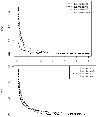
Figure 1. PDF Plots of LogLogi-Exponential Distribution

2.2.2. The LogLogi-Logistic Distribution. The Log-Logistic distribution has CDF and PDF as Η(υ)=(1+(λυ)^-β ) ^-1 and ℏ(υ)=λβ(λυ)^(β-1) (1+(λυ)^{^β} )^-2, respectively, with parameters λ and β. The CDF and PDF of the submodel denoted by LogLogi-Logistic (LogLogi-L) can be derived as



where υ>0 The β>0 is a shape parameter and  is a scale parameter.



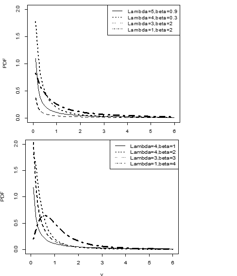
Figure 2. PDF Plots of LogLogi-Logistic Distribution

2.3. Estimation Methods

This section considers seven methods of estimation to estimate the unknown parameters of the LogLogi family of distributions. The estimation methods applied are (i) ML, (ii) LS, (iii) ωLS, (iv) PCE, (v) MPS, (vi) CVM, and (vii) ÅD.

2.3.1. Maximum Likelihood Estimation (MLE)Let ${\upsilon }_1,{\upsilon }_2,\dots ,{\upsilon }_n$ be the observed sample values from the LogLogi family of distributions having PDF $g(\upsilon ;\zeta )$.

The log-likelihood function is denoted by $L\left(\zeta \right|\overline{\upsilon })$ and written as:

$$L\left(\zeta \right|\overline{\upsilon })=nlog(0.5)+\sum _{i=1}^{n}logg({\upsilon }_i;\zeta )-0.5\sum _{i=1}^{n}logH({\upsilon }_i;\zeta )-0.5\sum _{i=1}^{n}log(1-H({\upsilon }_i;\zeta ))-2\sum _{i=1}^{n}log(\sqrt{H({\upsilon }_i;\zeta )}+\sqrt{1-H({\upsilon }_i;\zeta )})$$

By differentiating the log-likelihood function L(ζ|▁υ) with respect to parameter (s) ζ, we will get the normal equations. By solving these normal equations analytically or numerically, ML estimates of the proposed LogLogi family can be obtained.

2.3.2. Ordinary Least Squares (OLS)Consider a random sample of size $n$ from the LogLogi family of distribution, and let ${\upsilon }_{1:n}<{\upsilon }_{2:n}<\dots <{\upsilon }_{n:n}$ be the order observations.

Then we can obtain the LS estimates of the parameters of the LogLogi family of distributions by minimizing the expression:

$$S\left(\zeta \right)=\sum _{i=1}^n\left[H\right({\upsilon }_{i:n};\zeta )-\frac{i}{n+1}{]}^2$$

where $H(\upsilon ;\zeta )$ is a baseline CDF.

2.3.3. Weighted Least Squares (ωLS)Following the same notations as mentioned for OLS previously, the ωLS estimates can also be obtained by minimizing the expression:

$$\omega \left(\zeta \right)=\sum _{i=1}^n\frac{{(n+1)}^2(n+2)}{i(n-i+1)}\left[H\right({\upsilon }_{i:n};\zeta )-\frac{i}{n+1}{]}^2$$

where $H(\upsilon ;\zeta )$ is a baseline CDF.

2.3.4. Method of Percentile (PCE) To apply this method based on the quantile function, the key idea is to minimize the difference between sample percentiles and the theoretical percentiles derived from the distribution's quantile function.

Given the quantile function $Q(\nu ;\zeta )$ of the LogLogi distribution family with parameter(s) $\zeta$, the PCE estimates can be obtained by minimizing the following expression:

$$P\left(\zeta \right)=\sum _{i=1}^n[x_{i:n}-H^{-1}(\frac{\nu 2^{}}{\nu 2^{}+(1-\nu 2^{})},\zeta ){]}^2$$

where $0<\nu <1$.

2.3.5. Maximum Product of Spacing Method (MPS) Consider an ordered sample ${\upsilon }_{1:n}<{\upsilon }_{2:n}<\dots <{\upsilon }_{n:n}$ and the CDF $H(\upsilon ;\zeta )$ of the proposed LogLogi distribution family with parameter(s) $\zeta$. The MPS estimates of $\zeta$ are obtained by maximizing the product of spacings between these ordered sample points, defined as follows:

$$M\left(\zeta \right)=\frac{1}{n+1}\sum _{i=1}^{n+1}log{D}_i\left(\zeta \right)$$

where

$$D_i\left(\zeta \right)=H\left({\upsilon }_{i:n}\right|\zeta )-H({\upsilon }_{i-1:n}\left|\zeta \right)$$

where $H\left({\upsilon }_{0:n}\right|\zeta )=0$ and $H\left({\upsilon }_{n+1:n}\right|\zeta )=1$.

2.3.6. Method of Cram´er-von-Mises (CVM). The next two statistical techniques are often used for parameter estimation and goodness-of-fit testing. These quantify the difference between the sample data's empirical distribution function and the theoretical model.

Firstly, CVM is defined. Consider a sample observation ${\upsilon }_{1:n}<{\upsilon }_{2:n}<\dots <{\upsilon }_{n:n}$, sorted in ascending order, with a CDF $H(\upsilon ;\zeta )$ with parameter vector $\zeta$. The CVM estimates for $\zeta$ are obtained by minimizing $C\left(\zeta \right)$ with respect to $\zeta$:

$$C\left(\zeta \right)=\frac{1}{12n}+\frac{1}{n}\sum _{i=1}^n\left[H\right({\upsilon }_{i:n};\zeta )-\frac{2i-1}{2n}{]}^2$$

where ${\upsilon }_{i:n}$ denotes the $i^{th}$ order statistic in the sorted sample.

2.3.7. Method of Anderson-Darling (ÅD ). Following the mechanism of minimization, consider a sample observation υ_(1:n)<υ_(2:n)<...<υ_(n:n), , sorted in ascending order, with a CDFΗ(υ;ζ) with parameter vector ζ, the ÅD estimates for ζ are obtained by minimizing A(ζ)with respect to ζ

$$A\left(\zeta \right)=-n-\frac{1}{n}\sum _{i=1}^n(2i-1)\{\log H({\upsilon }_{i:n}\left|\zeta \right)+\log (1-H({\upsilon }_{n-i+1:n}\left|\zeta \right)\left)\right\},$$

, where v^i:n denotes

the i^th order statistic in the sorted sample.

3. SIMULATION STUDY OF THE LOGLOGI-E MODEL

The study undertook a M. Carlo simulation to evaluate the performance of the , , , , ,  and  estimation methods for the LogLogi-E distribution. For each parameter of the LogLogi-E model, the mean, bias, and mean square error were computed across varying sample sizes. These summaries measures were obtained by repeating the simulation process multiple times for each selected sample size. The simulated results of the LogLogi-E model at are given in Tables 1, 2, and 3.

As the sample sizes are increased, the mean simulated value tends to original supposed values. Additionally, the bias obtained by each method tends to zero as the sample sizes increase. Similar trends are also determined for the MSE of each method. The simulated results of the LogLogi-E model by each seven methods clearly show the consistency of the estimates and asymptotically unbiased.

3.1Data Analysis

To further assess its utility, the LogLogi family is explored through the LogLogi-L model with two real life datasets. First dataset refers to time-to-failure (in hours) of turbocharger used in a specific type of engine. Each from total 40 observations, representing the operational lifetime of the turbocharger until failure occur. It provides failure behavior and durability characteristics, making it useful for lifetime modeling.  This data set was used by Xu et al. [14]. The second dataset comprises the survival times (in months) of 20 patients who were diagnosed with acute myeloid leukemia. Each observation represents the duration from diagnosis to either death or the end of the study period, making it valuable for application in survival analysis and time event modeling. This data set was used by Afify et al. [15].

Table 1. Mean, Bias, and MSE of the LogLogi-E Model for

Method	Estimate	n=10	n=20	n=30	n=50	n=100	n=200	n=300
ML	Mean	1.88578	1.72263	1.608156	1.554885	1.532891	1.516067	1.508344
LS	Mean	2.107319	1.686933	1.6181	1.561735	1.529782	1.518896	1.509292
WLS	Mean	2.043634	1.656902	1.601244	1.552345	1.526236	1.516212	1.508554
CVM	Mean	2.193216	1.731717	1.648066	1.579366	1.538522	1.52324	1.512184
PCE	Mean	1.547705	1.44745	1.457001	1.44756	1.461672	1.473345	1.478725
MPS	Mean	1.537071	1.4428	1.457499	1.451449	1.469011	1.480471	1.484921
AD	Mean	1.803524	1.610383	1.581333	1.540953	1.521858	1.513609	1.506598
ML	Bias	0.38578	0.28748	0.108156	0.054885	0.032891	0.016067	0.008344
LS	Bias	0.607319	0.186933	0.1181	0.061735	0.029782	0.018896	0.009292
WLS	Bias	0.543634	0.156902	0.101244	0.052345	0.026236	0.016212	0.008554
CVM	Bias	0.693216	0.231717	0.148066	0.079366	0.038522	0.02324	0.012184
PCE	Bias	0.047705	-0.05255	-0.043	-0.05244	-0.03833	-0.02665	-0.02128
MPS	Bias	0.037071	-0.0572	-0.0425	-0.04855	-0.03099	-0.01953	-0.01508
AD	Bias	0.303524	0.110383	0.081333	0.040953	0.021858	0.013609	0.006598
ML	MSE	0.148827	0.102327	0.011698	0.003012	0.001082	0.000258	6.96E-05
LS	MSE	0.368837	0.034944	0.013948	0.003811	0.000887	0.000357	8.63E-05
WLS	MSE	0.295538	0.024618	0.01025	0.00274	0.000688	0.000263	7.32E-05
CVM	MSE	0.480549	0.053693	0.021924	0.006299	0.001484	0.00054	0.000148
PCE	MSE	0.002276	0.002761	0.001849	0.00275	0.001469	0.00071	0.000453
MPS	MSE	0.001374	0.003272	0.001806	0.002357	0.00096	0.000381	0.000227
AD	MSE	0.092127	0.012184	0.006615	0.001677	0.000478	0.000185	4.35E-05

Table 2. Mean, Bias, and MSE of the LogLogi-E Model for

Method	Estimate	n=10	n=20	n=30	n=50	n=100	n=200	n=300
ML	Mean	2.506317	2.366311	2.147423	2.077875	2.036928	2.021717	2.013743
LS	Mean	2.705231	2.249726	2.144788	2.073071	2.046248	2.025105	2.011243
WLS	Mean	2.626977	2.209806	2.122652	2.062773	2.041037	2.022577	2.010888
CVM	Mean	2.821682	2.310054	2.184035	2.096541	2.057951	2.030912	2.015082
PCE	Mean	2.036854	1.924847	1.931119	1.929103	1.949793	1.964953	1.970029
MPS	Mean	2.022736	1.918781	1.93136	1.934983	1.960314	1.975446	1.979414
AD	Mean	2.367672	2.149176	2.094102	2.051806	2.034288	2.018975	2.00842
ML	Bias	0.506318	0.250464	0.147424	0.077875	0.036928	0.021717	0.013743
LS	Bias	0.705231	0.249726	0.144788	0.073071	0.046248	0.025105	0.011243
WLS	Bias	0.626977	0.209806	0.122652	0.062773	0.041037	0.022577	0.010888
CVM	Bias	0.821682	0.310054	0.184035	0.096541	0.057951	0.030912	0.015082
PCE	Bias	0.036854	-0.07515	-0.06888	-0.0709	-0.05021	-0.03505	-0.02997
MPS	Bias	0.022736	-0.08122	-0.06864	-0.06502	-0.03969	-0.02455	-0.02059
AD	Bias	0.367672	0.149176	0.094102	0.051806	0.034288	0.018975	0.00842
ML	MSE	0.256357	0.104558	0.021734	0.006064	0.001364	0.000472	0.000189
LS	MSE	0.497351	0.062363	0.020964	0.005339	0.002139	0.00063	0.000126
WLS	MSE	0.393101	0.044019	0.015043	0.00394	0.001684	0.00051	0.000119
CVM	MSE	0.675161	0.096134	0.033869	0.00932	0.003358	0.000956	0.000227
PCE	MSE	0.001358	0.005648	0.004745	0.005026	0.002521	0.001228	0.000898
MPS	MSE	0.000517	0.006597	0.004711	0.004227	0.001575	0.000603	0.000424
AD	MSE	0.135183	0.022254	0.008855	0.002684	0.001176	0.00036	7.09E-05

Table 3. Mean, Bias, and MSE of the LogLogi-E Model for

Method	Estimate	n=10	n=20	n=30	n=50	n=100	n=200	n=300
ML	Mean	5.059087	4.759021	4.274531	4.164586	4.075315	4.041302	4.021166
LS	Mean	5.280128	4.533099	4.324273	4.142926	4.087729	4.044307	4.026456
WLS	Mean	5.137602	4.443417	4.279244	4.123711	4.077618	4.040633	4.024467
CVM	Mean	5.512552	4.652192	4.404179	4.190062	4.111037	4.055893	4.034232
PCE	Mean	4.052084	3.878288	3.864438	3.857835	3.89457	3.931908	3.943802
MPS	Mean	4.029397	3.865482	3.866626	3.870307	3.915234	3.951754	3.960795
AD	Mean	4.67171	4.317621	4.216967	4.099834	4.063382	4.033777	4.019242
ML	Bias	1.059087	0.59034	0.274531	0.164586	0.075315	0.041302	0.021166
LS	Bias	1.280128	0.533099	0.324273	0.142926	0.087729	0.044307	0.026456
WLS	Bias	1.137602	0.443417	0.279244	0.123711	0.077618	0.040633	0.024467
CVM	Bias	1.512552	0.652192	0.404179	0.190062	0.111037	0.055893	0.034232
PCE	Bias	0.052084	-0.12171	-0.13556	-0.14217	-0.10543	-0.06809	-0.0562
MPS	Bias	0.029397	-0.13452	-0.13337	-0.12969	-0.08477	-0.04825	-0.03921
AD	Bias	0.67171	0.317621	0.216967	0.099834	0.063382	0.033777	0.019242
ML	MSE	1.121666	0.121666	0.075367	0.027089	0.005672	0.001706	0.000448
LS	MSE	1.638727	0.284195	0.105153	0.020428	0.007696	0.001963	0.0007
WLS	MSE	1.294139	0.196619	0.077977	0.015304	0.006025	0.001651	0.000599
CVM	MSE	2.287813	0.425355	0.163361	0.036124	0.012329	0.003124	0.001172
PCE	MSE	0.002713	0.014814	0.018377	0.020211	0.011115	0.004637	0.003158
MPS	MSE	0.000864	0.018095	0.017789	0.01682	0.007185	0.002328	0.001537
AD	MSE	0.451194	0.100883	0.047074	0.009967	0.004017	0.001141	0.00037

The initial validation of the LogLogi-L model is to compare with competitive model by using real data. The important Log-logistics distribution is considered for comparison with the proposed LogLogi-L model. This is because, logistic distribution is being used as a special case in the LogLogi family. The following goodness-of-fit methods, namely, Kolmogorov–Smirnov (KS), Akaike Information Criterion (AIC), Bayesian Information Criterion (BIC), consistent Akaike Information Criterion (CAIC), and Hannan-Quinn Information Criterion (HQIC) were used for comparison. Model with smallest values of these statistics is deemed more suitable for the data. All the computations and graphs were performed by using the R software.

All goodness-of-fit statistics for the LogLogi-L and log-logistic model are summarized in Tables 4 and 5 for data 1 and 2. All four goodness-of-fit statistics presented in Table 4 have less values for the proposed LogLogi-L model than log-logistic distribution. Both datasets repeat the same results. This means that the LogLogi-L model outperforms than log-logistics model for both datasets 1 and 2. Hence, it can be inferred that the LogLogi-L model is a healthier (better) choice than log-logistic model. The study also outlined the Maximum Likelihood Estimates (MLEs) and their Standard Errors (SE) for the parameters of the LogLogi-L and log-logistics model in Table 5.

Table 4. Comparative Goodness-of-fit Results for the LogLogi-Logistic and Log-logistics Models

Data	Models	AIC	CAIC	HQIC	BIC
1	LogLogi-Logistic	2.659868	2.984192	6.037626	3.881159
	Log-logistic	3.84608	4.170404	7.223839	5.067371
2	LogLogi-Logistic	1.569319	2.275201	3.560784	1.958074
	Log-logistic	2.419614	3.125497	4.411079	2.808369

Table 5. The KS, MLEs, and Corresponding SE of the Models

Data	Models	Parameters	MLE	SE	KS
1	LogLogi-Logistic	λ̂	0.060759	0.08543	0.50203
		β̂	0.026936	0.08745	(3.50E-09)
	Log-logistic	λ̂	0.361183	0.294903	0.45072
		β̂	0.360601	0.294428	(1.75E-07)
2	LogLogi-Logistic	λ̂	0.011799	0.048632	0.50496
		β̂	0.012893	0.053186	(3.01E-05)
	Log-logistic	λ̂	0.278363	0.211494	0.49398
		β̂	0.280011	0.212759	(3.01E-05)

4. CONCLUSION

This study introduced a new and advanced flexible family of distributions that extends the corresponding parent distribution. Key features of the newly-developed family were derived. Furthermore, parameter estimation for the LogLogi family was explored using the familiar  method along with six additional estimation methods. The effectiveness of the LogLogi family is further demonstrated through the sub-model LogLogi-L, applied to two real-life datasets. The simulation results provided useful insights for the real-world applications where parameter estimation accuracy directly effects decision-making and model interpretation. Based on simulation results for three considered parameters, it was concluded that the  performed better than all other competitive models for small sample size, making it more suitable for empirical studies with limited or noisy data. Conversely, the  would be a better choice for large sample settings with well-behaved data distributions. These results may help policymakers, researchers, and analysts choose the most suitable estimation approach depending on data quality and study objects.

4.1. Future Research Directions

Future directions of the study should include the regression structure, specifically for the proposed sub-model. This is because the regression structure provides efficient results due to auxiliary information. Additionally, the proposed work can be extended for bivariate version. Moreover, the proposed study has some limitations. In particular, repeating the simulation study across a wider range of parameter combinations could provide deeper insights into estimator robustness. Furthermore, the Bayesian estimation can provide the better efficiency of the results.

CONFLICT OF INTEREST

The authors of the manuscript have no financial or non-financial conflict of interest in the subject matter or materials discussed in this manuscript.

DATA AVALIABILITY STATEMENT

The data is freely-available and the reference paper is cited in data analysis section.

FUNDING DETAILS

No funding was received for this research

REFERENCES

1. Pearson K. Contributions to the mathematical theory of evolution. Philos Trans R Soc Lond A. 1894;185:71–110.
2. Hastings C Jr, Mosteller F, Tukey JW, Winsor CP. Low moments for small samples: a comparative study of order statistics. Ann Math Stat. 1947;18:413–426. https://doi.org/10.1214/aoms/1177730388
3. Tukey JW. The Practical Relationship Between the Common Transformations of Percentages of Counts and of Amounts. Princeton University; 1960.
4. Azzalini A. A class of distributions which includes the normal ones. Scand J Stat. 1985;12:171–178.
5. Eugene N, Lee C, Famoye F. Beta-normal distribution and its applications. Commun Stat Theory Meth. 2002;31(4):497–512. https://doi.org/10.1081/STA-120003130
6. Zografos K, Balakrishnan N. On families of beta-generated and generalized gamma-generated distributions and associated inference. Stat Methodol. 2009;6(4):344–362. https://doi.org/10.1016/j.stamet.2008.12.003
7. Alzaatreh A, Lee C, Famoye F. A new method for generating families of continuous distributions. Metron. 2013;71(1):63–79. https://doi.org/10.1007/s40300-013-0007-y
8. Nassar M, Dey S, Kumar D. A new generalization of the exponentiated Pareto distribution with an application. Am J Math Manag Sci. 2018;37(3):217–242. https://doi.org/10.1080/01966324.2017.1396942
9. Shakhatreh MK, Lemonte AJ, Cordeiro GM. On the generalized extended exponential-Weibull distribution: properties and different methods of estimation. Int J Comput Math. 2020;97(5):1029–1057. https://doi.org/10.1080/00207160.2019.1605062
10. Sen S, Afify AZ, Al-Mofleh H, Ahsanullah M. The quasi xgamma-geometric distribution with application in medicine. Filomat. 2019;33(16):5291–5330. https://doi.org/10.2298/FIL1916291S
11. Afify AZ, Nassar M, Cordeiro GM, Kumar D. The Weibull Marshall–Olkin Lindley distribution: properties and estimation. J Taibah Univ Sci. 2020;14(1):192–204. https://doi.org/10.1080/16583655.2020.1715017
12. Nassar M, Afify AZ, Shakhatreh M. Estimation methods of alpha power exponential distribution with applications to engineering and medical data. Pak J Stat Oper Res. 2020;16(1):149–166. https://doi.org/10.18187/pjsor.v16i1.3129
13. Hassan EA, Elgarhy M, Eldessouky EA, Hassan OHM, Amin EA, Almetwally EM. Different estimation methods for new probability distribution approach based on environmental and medical data. Axioms. 2023;12(2):220. https://doi.org/10.3390/axioms12020220
14. Xu K, Xie M, Tang LC, Ho SL. Application of neural networks in forecasting engine systems reliability. Appl Soft Comput. 2003;2(4):255–268. https://doi.org/10.1016/S1568-4946(02)00059-5
15. Afify AZ, Nofal ZM, Butt NS. Transmuted complementary Weibull geometric distribution. Pak J Stat Oper Res. 2014;10(3):435–454. https://doi.org/10.18187/pjsor.v10i4.836