Price Volatility and Financial Performance: Assessing the Impact of Food Prices on Pakistan’s Industrial Sector

1. INTRODUCTION

The changes in food prices directly affect welfare of the consumers and producers because they alter resource availability and allocation. In this regard, changes in both demand and supply factors, cost of production and distribution, climate conditions and government policies are considered as the main sources of changes in the food prices (Dehghan et al., 2024). The rising food prices further result in inflation, reducing access to nutritional food due to eradication of purchasing power, and food insecurity particularly for the low-income consumers (Zhao et al., 2021). Similarly, the effect of rising food prices on the entrepreneurs across various industries can be traced through various channels such as rising input costs and production costs (Hendriks et al., 2023).

Pakistan as an agrarian country with rapidly growing population is facing serious challenges regarding the production, distribution and consumption of staple food. The availability as well as the affordability of the food items remain a challenge in Pakistan. These challenges are also linked with food security, social protection and economic development. Hence, it is quite imperative to analyze the implications of rising food prices on various stakeholders (Ollila, 2011). In Pakistan, the spike in global wheat, corn and soyabean prices in 2012 led to higher local food prices. Food prices became stable during the FY2014-15, but show the increasing trend in 2026 due to the rise in the wheat, sugar, meat and pulses.¹ During the FY 2018-19, global inflation remained moderate which alleviated the inflationary pressure causing the food inflation to drop to 1.8 percent.² Food prices continued to increase during covid-19 and food inflation remained in double digit during FY2019-20, FY 2020-21 and FY2021-22. The continuous increase in the food prices was mainly due to the country’s dependence on the imported commodities such as oil, tea, pulses and agricultural inputs as well as shortfall in the domestic production which also resulted in trade deficit. During this period, the food imports increased to USD 8 billion, while exports remained steady at USD 5.4 billion (Government of Pakistan, 2023). Overall, the fluctuations in food prices have serious implications in Pakistan where more than 40 percent of the population lives in poverty (World Bank, 2025). On the other hand, rising food prices also affect entrepreneurs’ decisions and business sustainability. Keeping in view the importance of food prices for the consumers’ demand and entrepreneurs’ supply decisions, this study aims to examine the effect of changes in food prices on the decisions made by consumers and entrepreneurs in Pakistan. This objective is answered through data analysis by using economic modelling. The findings of the study will provide insight to the policymakers to ensure food security measures, and enable the consumers and businesses to make informed decisions.

The structure of the paper is as follows: the literature of the study is reviewed in section 2, the methodology section discusses theories related to the study, the data collection process, and the statistical and analytical tools employed for analysis. We have presented and interpreted our research findings in the results and discussion section. Finally, in the conclusion and policy implication section, the paper summarizes key findings, their significance, and recommendations for policymakers and future researchers.

Literature Review

The relationship between the food prices, consumer behavior and producer decisions has the attention of researchers and policymakers. Particularly, how the rising food prices have critical implications for the low-income countries due to the larger share of the food expenditures in the household budget. Similarly, higher food prices also affect the decision of producers by altering their profit margins and production costs. A number of studies explore the impact of food prices on the consumers. The studies of Dehghan et al. (2024), Zhao et al. (2021), Waterlander et al. (2019), Yousif and Al-Kahtani, (2014) and Ollila (2011) confirm that rising food prices discourage food consumption and lower the nutritional quality. On the other hand, the studies of Timmer (2010), Subervie (2008) and Poulton et al. (2006) show the positive impact of higher food prices on the investment in agriculture sector, and negative impact on the investment in the food industry. The following section provides a critical analysis of the existing literature on the influence of food prices on consumer and entrepreneurial decision-making.

Recent literature highlights the food price dynamic’s effect on both demand and supply sides of industry markets. Dardeer and Shaheen (2025) study shows that food price inflation results from a combination of supply-side factors, such as production shocks and transportation issues, and demand-side pressures linked to income growth. It further affects the costs of making business and production decisions in the economy. In addition, Duru et al. (2024) argue that non-raw inputs such as energy and exchange rate fluctuations have a bidirectional linkage with food prices. Moreover, Türken and Yildirim’s (2024) study uses Bayesian SVAR model and highlights that food price inflation has the ability to significantly affect the aggregate inflation in Turkey economy.

Empirical work also investigates the impact of food price shocks on macro-economy. Israel and Charity (2024) examine the impact of food price shocks on the Nigerien economy and identify that prolonged food price shocks negatively affect the economic growth of the country. The study further revealed that food price shocks directly affect the purchasing power of consumers and indirectly affect the key macroeconomic variables such as interest rate and exchange rate. The study of price volatility shows that fluctuations in food prices negatively affect economic activity by introducing uncertainty into production planning, which discourages investments and impacts supply decisions (Wibowo et al., 2023).

The study of Engstrom and Eriksson (2023), estimates the price elasticity of various food products and explains the differences in the elasticities across diverse households by using the OLS estimation technique. The findings of the study identify a number of factors such shopping location, number of children, and use of organic products to influence the consumer behavior. This implies that food price changes provide valuable insight for policy decisions. Similarly, Waterlander et al. (2019) also analyze the impact of food prices on consumer preferences by using the monthly data from New Zealand. The sample consists of 4258 shops utilizing five tax and subsidy options. All the participants exposed to different food prices during various shopping occasions in the virtual supermarket setup. Results indicate that there is negligible effect of taxes on unhealthy food and subsidies on healthy food on the overall purchasing power of the consumers. The study of Yousif and Al-Kahtani (2014) observes the response of 286 households towards the rising prices in Saudi Arabia. The authors divide the sample on the basis of different income levels, and report that the rising food prices adversely affect the consumption of major food items, along with increasing the total expenditures of the households. The findings of the study suggest that the lower income groups are more vulnerable due to higher prices.

Ollila (2011) examines the food prices and consumer preferences to buy premium quality food items of Finnish consumers by developing a food price attitude scale through surveys. The findings of the study indicate that food price attitude is a multidimensional construct which can be positive or negative towards high and low food prices. Whereas, Zhao et al. (2021) focus on how food packaging and prices can affect the buying behavior of consumers while the customer’s satisfaction plays the mediating role. The study finds that there is a statistically significant relationship between product packaging, product price and consumer demand. Furthermore, customer satisfaction completely mediates product price while partially mediating the product packaging.

If we consider the supply side of the economy, the rising food prices encourage the reallocation of factors of production towards the food production sector. However, if the technology and inputs available at the farm gate level remain fixed then it limits the supply response (Asian Development Bank, 2008). Moreover, Poulton et al. (2006) find that food price volatility plays a critical role in the Eastern and Southern Africa by affecting the surplus and deficit households differently. The deficit households focus on the staple food while the surplus households prefer diversification and move to the higher value crops. In the context of Pakistan, Kurosaki and Fafchamps (2002), establish that the food production decision mainly depends on the support prices and yield risks. The study shows that if these risks are reduced then the cultivation area allocated for the cash crops can be increased up to 30 percent for the median farmers.

It is evident from the above discussion that food prices play a crucial role in shaping the consumers’ purchasing power and producers’ decisions. On the consumer side, the purchasing power of the consumers, consumer wellbeing, and consumption choices play a critical role. Higher prices discourage low-income consumers and force them to shift their consumption towards cheaper, lower-calorie food items, thereby affecting their well-being. Food price volatility also affects entrepreneurs by altering their production, pricing strategy, and product supply. Although studies have highlighted the impact of food prices on consumption and entrepreneurs (mainly in the food industry), no study directly captures the impact of food prices on industrial production and consumption. This study provides a novel analysis on the effect of food price on nine large scale manufacturing industries. The present study goes beyond the traditional analysis of food price shocks impact, and examines the role of food prices on the consumers’ and producers’ decisions through demand and supply channels. Overall, the study provides a detailed analysis of food price shocks impact to understand the challenges and opportunities available for the consumers as well as producers of large-scale manufacturing industries in Pakistan. The uneven distribution of income, households’ demographics, market conditions and culture barriers make Pakistan a unique case for the analysis purposes.

Methodology

The study used monthly data from June 2008 to June 2023 for nine selected large scale industries of Pakistan. Large scale industries play a significant role in the economic development of the country and have 8.2% share in total GDP. The industries are selected on the basis of the weight among the total large scale industries³.  Food prices include the prices of three sub-groups: food items⁴, alcoholic items, and tobacco^[5], hotels, and restaurants⁶. The weight of the Food Group in the Consumer Price Index (CPI) is 37.48%, which shows the importance of this group. Moreover, for lower-middle-income countries like Pakistan, food prices are a matter of great concern as Pakistan spends a significant portion of its income on food items. To examine the impact of food prices on industrial variables, we have taken two industry-specific variables: industrial output (iy) and industrial price (ip). The variables that represent the economic condition of the country are inflation (inf), short-run interest rate (ir), long-term interest rate (lr), aggregate production (y), and money supply (m)⁷.

The study used the Structural Vector Auto-regressive (SVAR) model to examine how food price shocks affect the nine manufacturing industries (large-scale) of Pakistan. SVAR model is the most appropriate model to analyze the impact of an unexpected shock in a dynamic model. Other estimation models, like ARDL, although work well in mixed order of integration, however, it is a single equation model and required the identification of a dependent variable that is not suitable for our study which focuses on the mutual endogeneity. On the other hand, the Jordan and Philips (2018) model is best for examining the long run impact and it does not incorporate the short run dynamics.

The SVAR model was identified using an information-based approach. This study used nine industries for analysis; therefore, for each industry, we will estimate a distinct SVAR model.

Following is the matrix form representation of our SVAR model:

The element in matrix A describes the contemporaneous relationship among the variables. Matrix  describes the relationship between the economic variables of the study and  among industry variables. The element  of matrix A describes the contemporaneous relationship among economic and industry variables and,  between industry and economic variables.

We have assumed that industry-specific variables, such as industrial output and price, have no specific impact on the economic variable of our economy (Jo et al., 2019). Therefore, the matrix  is equal to zero.

The components of the matrix A are estimated by the function of maximum likelihood for a specified matrix of covariance (obtained from the residuals of the macroeconomic block). To identify restrictions, we take guidance from Garzon and Hierro (2021); Lee and Ni (2002) and Sims and Zha (1998). We will estimate our macro base-line SVAR model separately (the element of  matrix); therefore, we first impose restrictions on the matrix

The highest number of parameters is 36⁸ in the matrix whereas the maximum independent movements in the covariance matrix is 21⁹; therefore, our macro base-line SVAR model requires at least 15¹⁰ fully identified restrictions.

Equation of long-term interest rate

In equation 8, we assume that food prices are set autonomously from the macroeconomic variables of our analysis (Ollila, 2011). On the other hand, the food prices are not included in the aggregate output equation as these prices are not directly related to industrial production. Further, we assumed that the goods market is independent of the money market variables. However, the equation of aggregate inflation incorporates the impact of output and food prices. Food prices directly affect money demand, as consumers in developing countries like Pakistan spend a large portion of their income on food items (Khan & Ahmed, 2004). Thus, equation 11 includes food prices and interest rate, which is the cost of holding money and income (Sims & Zha, 1998). The study assumes that the money supply equation is not affected by aggregate output and aggregate prices (Lee & Ni, 2002). The long-term r equation is the most endogenous of our macro-SVAR model and is assumed to be affected by all other macro variables of our analysis. We impose 16 restrictions to estimate our macroeconomic variables matrix,  . Thus, 20 parameters will be estimated with 21 independent movements of the covariance matrix (obtained through the residuals of macroblocks). Our model has one over identified restriction.

The elements in  of matrix A show the contemporary relationship of macro variables and industrial variables, and the matrix  displays the relationship of industrial variables. As mentioned earlier to get the precise effect of food price volatility, it is important to isolate them from the impact of macroeconomic shocks, so we treat the macro-economic shocks as exogenous. So, the industrial price and output equation can be written as follows:

Equation of industrial price

Equation of industrial output

Whereas for the elements of matrix are as follows:

The highest number of parameters is 4¹¹ in  whereas the maximum independent movements in the covariance matrix is 6¹²; therefore, our macro base-line SVAR model requires at least 1¹³ fully identified restriction. We have imposed the restriction on output equation following Lee and Ni (2002). We have estimated the reduced form SVAR for equation 16 and 17, and then rescaled our data of industrial price and output by dividing it with their Standard Deviations (SD) respectively. By applying scaling, the parameters β₁ and β₃ are adjusted to approximately equal unity. Subsequently, we proceed to estimate the SVAR model for scaled data, under the assumption that β₂ equals -θβ₄. Furthermore, the θ value is established to 2¹⁴. The categorization of our demand and supply equations hinges on the estimated coefficients' signs (β₂^ and β₄^), given the positive signs of β₁^ and β₃^. The rule of thumb is that if β₄^ shows a negative coefficient, we will treat equation 17 as a supply equation, whereas equation 16 characterizes our demand. Conversely, if β₄^ shows a positive coefficient, equation 17 denotes demand, and equation 16 signifies industrial supply.

The matrix with restriction is as follows;

Consequently, we undertake separate estimations of the aforementioned matrix for each industry. Estimating matrix  aids in discerning the pertinent industrial demand and supply dynamics. Once identified, these equations are augmented with the element matrix  revealing the simultaneous interplay between our industry-specific variables and macro variables. Given our primary focus on exploring the effects of commodity price shocks on the financial performance of the manufacturing sector, we treat all other macroeconomic variables as exogenous. Therefore, there will be three variables in the matrix   and it requires a minimum of 3 restrictions to meet the fully identified criteria.

Where food price is assumed to be set independently as mentioned earlier. Further we add restriction in equation 20 similar to equation 16.

We have imposed three restrictions and our model is just identified.

Results

This section presents the results of our analysis. Table 1, 2 and 3 present the results of Augmented Dicky Filler (ADF) test for industrial output, industrial prices and macro-economic variables respectively. Further, Schwarz Info Criterion (SIC) has been selected for the determination of lag length.

Table 1

Unit Root Test for Industrial Output Variables

Note. CV at 5% level with intercept=-2.88 and CV at 1% level with intercept=-3.48

Table 2

Unit Root Test for Industrial Price Variables

Note. CV at 5% level with intercept=-2.88 and CV at 1% level with intercept=-3.48

Table 3

Unit Root Test for Macro Variables

Note. CV at 5% level with intercept=-2.88 and CV at 1% level with intercept=-3.48

The literature review reveals that the SVAR model is estimated using two distinct approaches. The first method involves estimation at the level, irrespective of the stationarity of the data. Conversely, the second method involves using stationary data for estimation. The debate over which approach is more appropriate traces back to the seminal work of Sims (1976). Estimating with level data, regardless of stationarity, is noted to yield consistent estimators that are asymptotically normally distributed. However, conventional wisdom, as supported by standard textbooks, favors utilizing stationary data. This preference is driven by the notion that using stationary data aids in meeting the normality assumption, facilitating robust inference. Hence, our choice has been to employ stationary data for estimation.

Table 4

Identification of Demand and Supply

Table 4 shows that the coefficients of   are negative for automobile, electronics and fertilizer industries thus for these industries, 17 equations are for supply, and 16 equations are for demand. For all other industries,  is positive, therefore, 17 is our industrial demand equation while equation 16 is supply for these industries. After identification of demand and supply we will check the impulse response of food price on identified demand and supply. Figure 1 below shows the impulse response.

Figure 1

Impulse Responses to Food Price Shocks

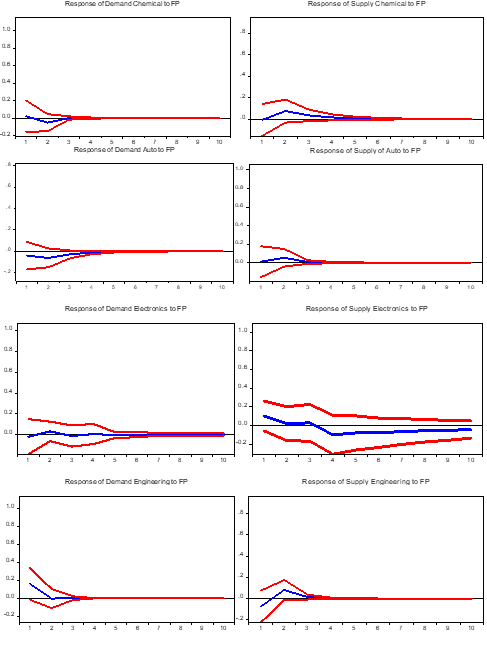
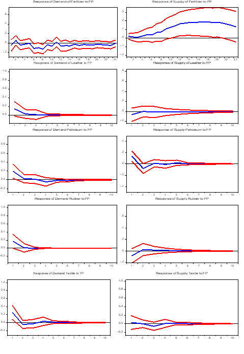
Table 5

Effect of Food Price Shocks

Note. The * represents the dominant responses are significant at 5%. “+” sign shows responses are positive and “-” shows response are negative. Mixed implies that positive and negative responses have similar magnitudes.

Figure 1 illustrates the dynamics of impulse responses to food price shocks. Additionally, Table 5 outlines these responses to identify how the food price affects the industrial demand and supply through the structural coefficient. The assessment of food price shock effects hinges on the relationship between industrial output and prices: when the output and prices move on the same side, the dominant effect is on the demand; conversely, when they move oppositely, it is on the supply. Additionally, whether the impact is positive or negative depends on the patterns within impulse responses.

Food is a necessity for human survival; consumers generally spend a significant portion of their income on it. Therefore, an increase in food prices directly affects the purchasing power of consumers and as a result, it reduces the demand for durable automobiles (Lambert & Miljkovic, 2010). Further, it also affects the demand for durable through income effect (Fadhilah et al., 2020) and precautionary saving effect due to uncertainty resulting from food price shocks (Engstrom & Eriksson, 2023). The food price shocks increase the supply of chemical industries significantly; however, it has insignificant impact on demand. The high price of food reduces aggregate demand in the short run and causes excess supply in the chemical industry.

Food price shocks have no significant impact on the electronic industry. Food price shocks, whether they lead to increases in demand or supply, have a positive impact on the engineering industry. These results are inconsistent with the finding of Bonilla-Cedrez et al. (2021) who assert that food price shocks negatively impact the demand of durable. In Pakistan, however, the engineering sector has long been overlooked and beset by numerous challenges. These include persistent energy crises, volatile policies, political instability, brain drain, and a lack of demand for locally manufactured goods. Nonetheless, the government of Pakistan has set forth an ambitious vision for 2030, aiming to raise the industrial production share to 30% of the GDP. To realize this objective, significant efforts have been made to bolster the engineering industry and enhance production capabilities that made this industry strong enough to respond towards the shocks in commodity prices like food.

The shocks in food prices increased the supply of fertilizer industry in the short run, however, this impact is not stable in the long run. The increased food prices provide farmers with a strong incentive to boost their production in order to capitalize on the improved profitability. To achieve greater yields, farmers often escalate their utilization of agricultural inputs such as fertilizers to enhance soil fertility and crop productivity (Hendriks et al., 2023).  Additionally, the prospect of higher profits can prompt farmers to consider expanding their cultivated land to accommodate more crops. The food price shocks have an insignificant impact on the leather industry. Whereas, it provides mixed results for petroleum because most of the petroleum products are used as inputs in the production of final food items. Further, the food price shocks increase the demand of rubber and textile industry in the short run and the model is stable in the long run.

Conclusion

 Food price volatility has the potential to affect the household consumption pattern and, as a result, the firms' manufacturing decisions. This study addressed this dimension of food price volatility, and it examines how food price volatility affects the financial performance of the manufacturing sector through its demand and supply channels. It used monthly data from June 2008 to June 2023 for nine selected large scale industries of Pakistan and employed the SVAR model for analysis.

Food price shocks, like other commodity price shocks, follow a ratchet effect where the increase in food prices have multiple effects on the economy. The decrease in the food price generally does not follow the same path. Therefore, in our analysis, we focus on the single positive direction.  Figure 2 below concludes the findings of our study.

Figure 2

Summarized Results of Food Price Shocks

Overall food price shocks show a positive impact on industries, and demand side impact is more dominating. Further, it is also interesting to note that food price shocks present the same pattern of response, and the responses are short lived for almost all industries. This short-lived response, that occurs in the initial months in industrial prices and output, is due to the nature of our data that took the monthly year adjusted variations. Understanding these dynamics of food price shocks enables policymakers to create targeted strategies for stabilizing the economy and fostering sustainable growth in Pakistan's manufacturing sector. Additionally, investors can make informed decisions, and industry stakeholders can adjust their strategies to address challenges and capitalize on opportunities presented by fluctuating food prices.

The study is subject to a few limitations. The data constraints preclude an analysis of how demand and supply adjust at firm or industry levels following the food price shocks. Additionally, the study does not try to differentiate short-run adjustment mechanisms from long-run ones in regard to industrial production. However, this study provides a pathway to future studies that can use panel data at the industry or firm level to evaluate how food price shocks transmit along the industrial supply chain. Additionally, further research can examine how food price changes driven by demand factors differ from those caused by supply shocks in terms of their impacts on industrial production, fixed investment and employment.

Author Contribution

Humera Irum: conceptualization, data curation, formal analysis, writing – original draft, methodology, supervision. Abida Yousaf: writing – review & editing, software, investigation, validation, visualization

Conflict of Interest

The authors of the manuscript have no financial or non-financial conflict of interest in the subject matter or materials discussed in this manuscript.

Data Availability Statement

Data supporting the findings of this study will be made available by the corresponding author upon request.

Funding Details

No funding has been received for this research.

Generative AI Disclosure Statement

The authors did not used any type of generative artificial intelligence software for this research.

REFERENCES

Asian Development Bank. (2008). Food prices and inflation in developing Asia: Is poverty reduction coming to an end? Asian Development Bank.
Bonilla-Cedrez, C., Chamberlin, J., & Hijmans, R. J. (2021). Fertilizer and grain prices constrain food production in sub-Saharan Africa. Nature Food, 2(10), 766–772. https://doi.org/10.1038/s43016-021-00370-1
Dardeer, M. & Shaheen, R. (2025). Structural determinants of food price inflation and food security implications: Evidence from GCC panel data. Humanities and Social Sciences Communications, 12, Article e1877. https://doi.org/10.1057/s41599-025-06148-1
Dehghan, M., Moosavi, S. N., & Zare, E. (2024). Analyzing the impact of government subsidies on household welfare during economic shocks: A case study of Iran. Bio-based and Applied Economics, 13(4), 387–396. https://doi.org/10.36253/bae-15105
Duru, S., Çelik, H., Hayran, S., & Gül, A. (2024). The relationship between food prices and non-raw material inputs: Evidence from VAR analysis. International Journal of Economics, Management and Accounting, 32(1), 203–216. https://doi.org/10.31436/ijema.v32i1.1187
Engström, F., & Eriksson, C. (2023). Impact of increased grocery prices on households: Studying Sweden 2022/2023 (Master's Thesis). KTH Royal Institute of Technology. https://kth.diva-portal.org/smash/record.jsf?pid=diva2:1773264
Fadhilah, E. F., & Ayu, S. F. (2020, February). The effect of food commodity price fluctuations on inflation in Pematang Siantar City. In IOP Conference Series: Earth and Environmental Science (Vol. 454, No. 1, p. 012019). IOP Publishing. https://doi.org/10.1088/1755-1315/454/1/012019
Garzon, A. J., & Hierro, L. A. (2021). Asymmetries in the transmission of oil price shocks to inflation in the eurozone. Economic Modelling, 105, Article e105665. https://doi.org/10.1016/j.econmod.2021.105665
Government of Pakistan, Ministry of Finance. (2023). Inflation (Chapter 7). In Pakistan Economic Survey 2022-23. Government of Pakistan. https://finance.gov.pk/survey/chapters_23/07_Inflation.pdf
Hendriks, S., de Groot Ruiz, A., Acosta, M. H., Baumers, H., Galgani, P., Mason-D'Croz, D., & Watkins, M. (2023). The true cost of food: A preliminary assessment. In Science and innovations for food systems transformation (pp. 581-601). Cham: Springer International Publishing. https://doi.org/10.1007/978-3-031-15703-5_32
Israel, K. E., & Charity, G. (2024). Food inflation and the Nigerian economy: An empirical investigation. International Journal of Research and Innovation in Social Science, 8(11), 3455–3465. https://doi.org/10.47772/IJRISS.2024.8110266
Jordan, S., & Phillips, A. Q. (2018). Dynamic simulation and testing for single-equation cointegrating and stationary autoregressive distributed models. The R Journal, 10(2), 469–488. https://doi.org/10.32614/RJ-2018-076
Khan, M. A., & Ahmed, A. (2014). Revisiting the macroeconomic effects of oil and food price shocks to Pakistan economy: A structural vector autoregressive (SVAR) analysis. OPEC Energy Review, 38(2), 184–215. https://doi.org/10.1111/opec.12020
Kurosaki, T., & Fafchamps, M. (2002). Insurance market efficiency and crop choices in Pakistan. Journal of Development Economics, 67(2), 419–453. https://doi.org/10.1016/S0304-3878(01)00188-2
Lambert, D. K., & Miljkovic, D. (2010). The sources of variability in US food prices. Journal of Policy Modeling, 32(2), 210–222. https://doi.org/10.1016/j.jpolmod.2010.01.001
Lee, K., & Ni, N. (2002). On the dynamic effects of oil price shocks: A study using industry level data. Journal of Monetary Economics, 49(4), 823–852. https://doi.org/10.1016/S0304-3932(02)00114-9
Ollila, S. (2011). Consumers' attitudes towards food prices (Doctoral Dissertation, Department of Economics and Management, University of Helsinki). University of Helsinki, 1–340. https://helda.helsinki.fi/handle/10138/28240
Poulton, C., Kydd, J., Wiggins, S., & Dorward, A. (2006). State intervention for food price stabilisation in Africa: Can it work? Food Policy, 31(4), 342–356. https://doi.org/10.1016/j.foodpol.2006.02.004
Sims, C. A. (1976). Econometric models and causal relations. American Economic Review, 66(2), 312–320.
Sims, C. A., & Zha, T. (1998). Bayesian methods for dynamic multivariate models. International Economic Review, 39(4), 949–968. https://doi.org/10.1111/1468-2354.00054
Subervie, J. (2008). The variable response of agricultural supply to world price instability in developing countries. Journal of Agricultural Economics, 59(1), 72–92. https://doi.org/10.1111/j.1477-9552.2007.00136.x
Timmer, C. P. (2010). Reflections on food crises past. Food Policy, 35(1), 1–11. https://doi.org/10.1016/j.foodpol.2009.09.002
Türken, F., & Yildirim, O. (2024). Second‑round effects of food prices on core inflation in Turkey. Economics and Business Review, 10(4), 32–55. https://doi.org/10.18559/ebr.2024.4.1485
Waterlander, W. E., Jiang, Y., Nghiem, N., Eyles, H., Wilson, N., Cleghorn, C., & Blakely, T. (2019). The effect of food price changes on consumer purchases: a randomised experiment. The Lancet Public Health, 4(8), e394–e405. https://doi.org/10.1016/S2468-2667(19)30105-7
Wibowo, H. E., Novanda, R. R., Ifebri, R., & Fauzi, A. (2023). Food price volatility and its implications for production and investment decisions: A review of the literature. AGRITROPICA: Journal of Agricultural Sciences, 6(1), 22–32. https://doi.org/10.31186/j.agritropica.6.1.22-32
World Bank. (2025, April 23). Pakistan's poverty rate to stand at 42.4%. Business Recorder. https://www.brecorder.com/news/40359069/pakistans-poverty-rate-to-stand-at-42-4-world-bank/
Yousif, I. E. A. K., & Al-Kahtani, S. H. (2014). Effects of high food prices on consumption pattern of Saudi consumers: A case study of Al Riyadh city. Journal of the Saudi Society of Agricultural Sciences, 13(2), 169–173. https://doi.org/10.1016/j.jssas.2013.05.003
Zhao, H., Chang, J., Havlík, P., van Dijk, M., Valin, H., Janssens, C., & Obersteiner, M. (2021). China's future food demand and its implications for trade and environment. Nature Sustainability, 4(12), 1042–1051. https://doi.org/10.1038/s41893-021-00784-6
1Economic Survey of Pakistan, 2012-2013; 2013-2014 and 2015-2016.
2Pakistan Bureau of Statistics, several publications from 2018 to 2019.
3Approximately 60 % of large scale manufacturing industries.
4Food and non- Alcoholic beverages include the price of 39 basic food commodities.
5Tobacco include the price of cigarettes and betel leaves and nuts.
6Hotel and restaurants include price of ready-made food.
7The data of all the variables are converted to the year- to -year monthly average data because the industry output data is collected from QIM issued by the PBS. The following QIM formula is used for the data (Output of nth industry in July 2009)/(Output of nth industry in July 2008) *(100-100)
8 k2
9 k(k+1)/2
10k(k-1)/2
11 k2
12 k(k+1)/2
13k(k-1)/2
14It has been checked that change in the value of θ does not impact our results.